CIAtah one-page README¶

This page contains all the documents in a single page and is automatically updated to reflect the current state of each page.

—Setup—

¶

Quick start guide¶

Below are steps needed to quickly get started using the CIAtah software package in MATLAB.

Install¶

• Clone the CIAtah repository (using GitHub desktop or command line) or download the repository zip and unzip (e.g. run below MATLAB command).

• Point the MATLAB path to the CIAtah root folder (NOT @ciatah sub-folder in the repository).

  • Alternatively, download the package from File Exchange using the Add-Ons explorer in MATLAB. See CIAtah entry at:

or https://www.mathworks.com/matlabcentral/fileexchange/75466-calciumimaginganalysis.

% Optional: this will set MATLAB working folder to the default user path. Make sure you have read/write permissions.

try; cd(userpath); catch; end;



% Download and unzip current repository

unzip('https://github.com/bahanonu/ciatah/archive/master.zip');



% Make CIAtah the working folder

cd('ciatah-master')

Check required toolboxes installed¶

CIAtah depends on several MATLAB toolboxes to run properly. Run the below command to have CIAtah check whether dependencies have been installed properly. If not use the Add-Ons (https://www.mathworks.com/help/matlab/matlab_env/get-add-ons.html) explorer to install each toolbox.

ciapkg.io.matlabToolboxCheck;`

Setup CIAtah¶

• Run CIAtah using the below MATLAB commands. Call obj; in the MATLAB command window each time you want to go back to the main GUI. Note: calciumImagingAnalysis class is now called ciatah, all functionality is the same.

% Run these commands in MATLAB to get started.



% Loads the class into an object for use in this session

obj = ciatah;



% Runs routines to check dependencies and help user get setup.

obj.setup;



% Open the class menu (always type `obj` then enter load the class/modules menu)

obj % then hit enter, no semicolon!

• Afterwards, likely want to run modelAddNewFolders module first in order to add folders containing imaging data to the current class object.

• [Optional] Users on Windows systems should download Everything (https://www.voidtools.com/). It is a very useful and extremely fast search engine for files and folders on a computer that can allow users to quickly get lists of folders then need to analyze in CIAtah.

• [Optional] Users who want to run analysis via the command line can run edit ciapkg.demo.cmdLinePipeline and run each segment of code there to see what commands are needed to perform each step. It assumes you have already run example_downloadTestData.

CIAtah main GUI notes¶

• All main decisions for choosing a method/procedure to run, cell-extraction algorithm, and which folders to analyze are in a single window.

• The GUI will real-time update the selected folders based on the selections in the subject, assay, and folder filter areas.

• Sections not relevant for a specific method are grayed out.

• Tab to cycle through selection areas. Green background is the currently selected area, dark gray background is area that had previously been selected but is not the active area, and white background is for areas that have not been selected yet.

• Hover mouse over method names for tooltip that gives additional information.

For example, selecting middle two assays automatically changes selection in Loaded folders section.

Certain sections become available when user selects the appropriate method (e.g. cell-extraction method available when selecting modelExtractSignalsFromMovie).

Additional quick start notes¶

• See additional details in Processing calcium imaging data for running the full processing pipeline.

• Settings used to pre-process imaging movies (modelPreprocessMovie module) are stored inside the HDF5 file to allow CIAtah to load them again later.

• To force load all directories, including most external software packages (in _external_programs folder), type ciapkg.loadAllDirs; into MATLAB command line. This is most relevant when you need to access specific functions in an outside repository that are normally hidden until needed.

• When issues are encountered, first check the *Common issues and fixes Wiki page to see if a solution is there. Else, submit a new issue or email Biafra (bahanonu [at] alum.mit.edu).

• Notes:

  • There are two sets of test data that are downloaded:

    • Single session analysis: data\2014_04_01_p203_m19_check01_raw can be used to test the pipeline until the cross-session alignment step.
    • Batch analysis: data\batch contains three imaging sessions that should be processed and can then be used for the cross-session alignment step. Users should try these sessions to get used to batched analysis.

  • For Fiji dependency, when path to Miji.m (e.g. \Fiji.app\scripts folder) is requested, likely in \_external_programs\FIJI_FOLDER\Fiji.app\scripts where FIJI_FOLDER varies depending on OS, unless the user requested a custom path or on OSX (in which case, find Fiji the install directory).

    • If you run into Java heap space memory errors when Miji tries to load Fiji in MATLAB, make sure "java.opts" file is in MATLAB start-up folder or that CIAtah folder is the MATLAB start-up folder (instructions on changing).

  • CIAtah often uses regular expressions to find relevant movie and other files in folders to analyze.

    • For example, by default it looks for any movie files in a folder containing concat, e.g. concat_recording_20140401_180333.h5 (test data). If you have a file called rawData_2019_01_01_myInterestingExperiment.avi and all your raw data files start with rawData_ then change the regular expression to rawData_ when requested by the repository. See setMovieInfo module to change after adding new folders.
  • CIAtah generally assumes users have imaging data associated with one imaging session and animal in a given folder. Follow folder naming conventions in Data for best experience.
  • External software packages are downloaded into _external_programs folder and should be placed there if done manually.

Users can alternatively run setup as below.

% Run these commands in MATLAB to get started.



% Loads all directories

loadBatchFxns;



% Loads the class into an object for use in this session

obj = ciatah;



% Download and load dependent software packages into "_external_programs" folder.

% Also download test data into "data" folder.

% Normally only need to one once after first downloading CIAtah package.

obj.loadDependencies;



% Add folders containing imaging data.

obj.modelAddNewFolders;



% [optional] Set the names CIAtah will look for in each folder

obj.setMovieInfo;



% Open class menu to pick module to run.

obj.runPipeline; % then hit enter!

Installation¶

Note, this is an alternative method of installation to that outlined in Quick Start.

Clone the CIAtah repository or download the repository zip and unzip.

• Point the MATLAB path to the CIAtah folder.

• Run loadBatchFxns.m before using functions in the directory. This adds all needed directories and sub-directories to the MATLAB path.

• Type obj = ciatah; into MATLAB command window and follow instructions that appear after to add data and run analysis.

• Run the ciatah class method loadDependencies or type obj.loadDependencies after initializing a ciatah object into the command window to download and add Fiji to path, download CNMF/CNMF-E repositories, download/setup CVX (for CNMF/CNMF-E), and download example data.

Note

• Place CIAtah in a folder where MATLAB will have write permissions, as it also creates a private subdirectory to store some user information along with downloading required external software packages.

• file_exchange folder contains File Exchange functions used by CIAtah.

• In general, it is best to set the MATLAB startup directory to the CIAtah folder. This allows java.opts and startup.m to set the correct Java memory requirements and load the correct folders into the MATLAB path.

• If CIAtah IS NOT the startup folder, place java.opts wherever the MATLAB startup folder is so the correct Java memory requirements are set (important for using ImageJ/Miji in MATLAB).

• If it appears an old CIAtah repository is loaded after pulling a new version, run restoredefaultpath and check that old CIAtah folders are not in the MATLAB path.

Example data¶

The CIAtah repository contains several example one-photon calcium imaging movies from miniature microscope experiments in freely moving rodents.

To download example data, run loadDependencies module (e.g. obj.loadDependencies) and select Download test one-photon data. option to download one-photon miniature microscope example datasets to use for testing CIAtah preprocessing, cell extraction, and cell classification code. The data will be located in the data folder within the repository root directory.

Else run example_downloadTestData.m from the MATLAB command line with the working directory set to the CIAtah repository.

Dependencies¶

By default external MATLAB-based software packages are stored in _external_programs.

MATLAB Toolbox dependencies¶

• Primary toolboxes

  • distrib_computing_toolbox
  • image_toolbox
  • signal_toolbox
  • statistics_toolbox

• Secondary toolboxes (not required for main pre-processing pipeline)

  • video_and_image_blockset
  • bioinformatics_toolbox
  • financial_toolbox
  • neural_network_toolbox

Parallel Computing Toolbox (PCT)¶

By default both CIAtah and PCT auto-start a parallel pool for functions that use parallelization (e.g. or calls to parfor). For some users this may not be desired, in that case go to MATLAB preferences and uncheck the below.

Or enter the following commands into the MATLAB command window:

parSet = parallel.Settings;

parSet.Pool.AutoCreate = false;

ImageJ¶

• Run downloadMiji from downloads\downloadMiji.m or obj.loadDependencies (when class initialized) to download Fiji version appropriate to your platform.

• Else download Fiji (preferably 2015 December 22 version): https://imagej.net/Fiji/Downloads.

• Make sure have Miji in Fiji installation: http://bigwww.epfl.ch/sage/soft/mij/.

• This is used as an alternative to the CIAtah playMovie.m function for viewing movies and is needed for some movie modification steps.

Saleae¶

• Only download if doing behavior and imaging experiments that use this DAQ device to collect data.

• Download 1.2.26: https://support.saleae.com/logic-software/legacy-software/older-software-releases#1-2-26-download.

CNMF and CNMF-E¶

• Download repositories by running downloadCnmfGithubRepositories.m or obj.loadDependencies (when class is initialized).

• CNMF: https://github.com/flatironinstitute/CaImAn-MATLAB.

• CNMF-E: https://github.com/bahanonu/CNMF_E

  • forked from https://github.com/zhoupc/CNMF_E to fix HDF5, movies with NaNs, and other related compatibility issues.

• CVX: http://cvxr.com/cvx/download/.

  • Download All platforms (Redistributable: free solvers only), e.g. http://web.cvxr.com/cvx/cvx-rd.zip.

Neurodata Without Borders¶

Neurodata Without Borders (NWB) file support requires the following GitHub repositories be present in the _external_programs folder. These are downloaded automatically when running obj.setup.

• https://github.com/schnitzer-lab/nwb_schnitzer_lab.

• https://github.com/ewiger/yamlmatlab.

• https://github.com/NeurodataWithoutBorders/matnwb.

—Repository—

¶

Data¶

The class generally operates on the principal that a single imaging session is contained within a single folder or directory. Thus, even if a single imaging session contains multiple trials (e.g. the imaging data is split across multiple movies) this is fine as the class will concatenate them during the preprocessing step should the user request that.

The naming convention in general is below. Both TIF and AVI raw files are supported and are converted to HDF5 after processing since that format offers more flexibility during cell extraction and other analysis steps.

Input and output files¶

• Default raw imaging data filename: concat_.*.(h5|tif).

• Default raw processed data filename: folderName_(processing steps).h5, where folderName is the directory name where the calcium imaging movies are located.

• Main files output by CIAtah. Below, .* normally indicates the folder name prefixed to the filename.

  • .*_pcaicaAnalysis.mat: Where PCA-ICA outputs are stored.
  • .*_ICdecisions_.*.mat: Where decisions for cell (=1) and not cell (=0) are stored in a valid variable.
  • .*_regionModSelectUser.mat: A mask of the region (=1) to include in further analyses.
  • .*_turboreg_crop_dfof_1.h5: Processed movie, in this case motion corrected, cropped, and Δ_F/F_.
  • processing_info: a folder containing preprocessing information.

Loading data¶

Users can load data from any NWB or CIAtah-style MAT files containing cell-extraction outputs using the ciapkg.io.loadSignalExtraction function as below.

[inputImages,inputSignals,infoStruct,algorithmStr,inputSignals2] = ciapkg.io.loadSignalExtraction(fileName);

NWB Support¶

CIAtah supports NWB format and by default will output cell-extraction analysis as CIAtah format unless user specifies otherwise. NWB files are by default stored in the nwbFiles sub-folder. This can be changed by setting the obj.nwbFileFolder property to a different folder name. Learn more about saving and loading

• Default image mask HDF5 dataset name: /processing/ophys/ImageSegmentation/PlaneSegmentation.

• Default fluorescence activity HDF5 dataset name: /processing/ophys/Fluorescence/RoiResponseSeries.

Preferred folder naming format¶

Folders should following the format YYYY_MM_DD_pXXX_mXXX_assayXX_trialXX where:

• YYYY_MM_DD = normal year/month/day scheme.

• pXXX = protocol number, e.g. p162, for the set of experiments performed for the same set of animals.

• mXXX = subject ID/number, e.g. m805 or animal ID.

• assayXX = assay ID and session number, e.g. vonfrey01 is the 1st von Frey assay session.

• trialXX = the trial number of the current assay session, only applicable if multiple trials in the same assay session.

Videos¶

• HDF5:

  • Saved as a [x y t] 3D matrix where x and y are the height and width of video while t is number of frames.
  • /1 as the name for directory containing movie data.
  • HDF can be read in using Fiji, see http://lmb.informatik.uni-freiburg.de/resources/opensource/imagej_plugins/hdf5.html.
  • Each HDF5 file should contain imaging data in a dataset name, e.g. /1 is the default datasetname for [x y frames] 2D calcium imaging movies in this repository.
  • Most functions have a inputDatasetName option to specify the dataset name if different from /1.

• TIF

  • Normal [x y frames] tif.

• AVI

  • Raw uncompressed grayscale [x y frames] avi.

Cell images¶

• IC filters from PCA-ICA and images from CNMF(-E).

  • [x y n] matrix
  • x and y being height/width of video and n is number of ICs output.

Cell traces¶

• IC traces from PCA-ICA and images from CNMF(-E).

  • [n f] matrix.
  • n is number of ICs output and f is number of movie frames.

  Repository notes¶

  • Covers preprocessing of calcium imaging videos, cell and activity trace extraction (supports the following methods: PCA-ICA, CELLMax, EXTRACT, CNMF, CNMF-E, and ROI), manual and automated sorting of cell extraction outputs, cross-session alignment of cells, and more.

• Supports PCA-ICA, CNMF, CNMF-E, EXTRACT, and ROI cell extraction methods publicly along with CELLMax for Schnitzer Lab collaborators. Additional methods can be integrated upon request.

• Most extensively tested on Windows MATLAB 2018b and 2019a. Moderate testing on Windows MATLAB 2015b, 2017a, 2017b, and 2018b along with OSX (10.10.5) 2017b and 2018b. Individual functions and CIAtah class should work on other MATLAB versions after 2015b, but submit an issue if errors occur. Newer MATLAB version preferred.

• This repository consists of code used in and released with

  • G. Corder, __B. Ahanonu__, B. F. Grewe, D. Wang, M. J. Schnitzer, and G. Scherrer (2019). An amygdalar neural ensemble encoding the unpleasantness of painful experiences. Science, 363, 276-281. http://science.sciencemag.org/content/363/6424/276.

  • and similar code helped process imaging or behavioral data in:

    • J.G. Parker, J.D. Marshall, B. Ahanonu, Y.W. Wu, T.H. Kim, B.F. Grewe, Y. Zhang, J.Z. Li, J.B. Ding, M.D. Ehlers, and M.J. Schnitzer (2018). Diametric neural ensemble dynamics in parkinsonian and dyskinetic states. Nature, 557, 177–182. https://doi.org/10.1038/s41586-018-0090-6.
    • Y. Li, A. Mathis, B.F. Grewe, J.A. Osterhout, B. Ahanonu, M.J. Schnitzer, V.N. Murthy, and C. Dulac (2017). Neuronal representation of social information in the medial amygdala of awake behaving mice. Cell, 171(5), 1176-1190. https://doi.org/10.1016/j.cell.2017.10.015.

• Code mostly developed while in Prof. Mark Schnitzer's lab at Stanford University. Credit to those who helped in Acknowledgments.

• Please check the 'Wiki' for further instructions on specific processing/analysis steps and additional information of software used by this package.

• When issues are encountered, first check the Common issues and fixes Wiki page to see if a solution is there. Else, submit a new issue.

Repository organization¶

Below are a list of the top-level directories and what types of functions or files are within.

• __@ciatah - Contains ciatah class and associated methods for calcium imaging analysis.

• externalprograms_ - External software packages (e.g. CNMF, CELLMax, and others) are stored here.

• +ciapkg - Package containing CIAtah functions. All functions will eventually be moved here to create a clean namespace.

• ciapkg

  - overloaded - Functions that overload core MATLAB functions to add functionality or fix display issues.

  - behavior - Processing of behavior files (e.g. accelerometer data, Saleae files, etc.).

  - classification - Classification of cells, e.g. manual classification of cell extraction outputs or cross-session grouping of cells.

  - data - Location of test data.

  - download - Functions that help download external code packages or data.

  - file_exchange - Contains any outside code from MATLAB's File Exchange that are dependencies in repository functions.

  - hdf5 - Functions concerned with HDF5 input/output.

  - image - Functions concerned with processing images (or [x y] matrices).

  - inscopix - Functions concerned with Inscopix-specific data processing (e.g. using the ISX MATLAB API).

  - io - Contains functions concerned with file or function input-output.

  - motion_correction - Functions concerned with motion correction.

  - movie_processing - Functions concerned with preprocessing calcium imaging videos, e.g. spatial filtering, downsampling, etc.

  - neighbor - Detection and display of neighboring cell information.

  - private - This directory contains various user settings, output pictures/data/logs from CIAtah modules, and more. This directory is NOT included in the MATLAB path, hence is good for storing related scripts without interfering with CIAtah.

  - python - Python code, e.g. for processing Saleae data.

  - serial - Code for saving and processing serial port data, e.g. Arduino streaming data.

  - settings - Functions concerned with settings for other functions.

  - signal_extraction - Functions related to cell extraction, e.g. running PCA-ICA.

  - signal_processing - Functions to process cell activity traces.

  - tracking - ImageJ and MATLAB functions to track animal location in behavior movies.

  - unit_tests [optional] - Functions to validate specific repository functions.

  - video - Functions to manipulate or process videos, e.g. making movie montages or adding dropped frames.

  - view - Functions concerned with displaying data or information to the user, normally do not process data.

—Processing data—

¶

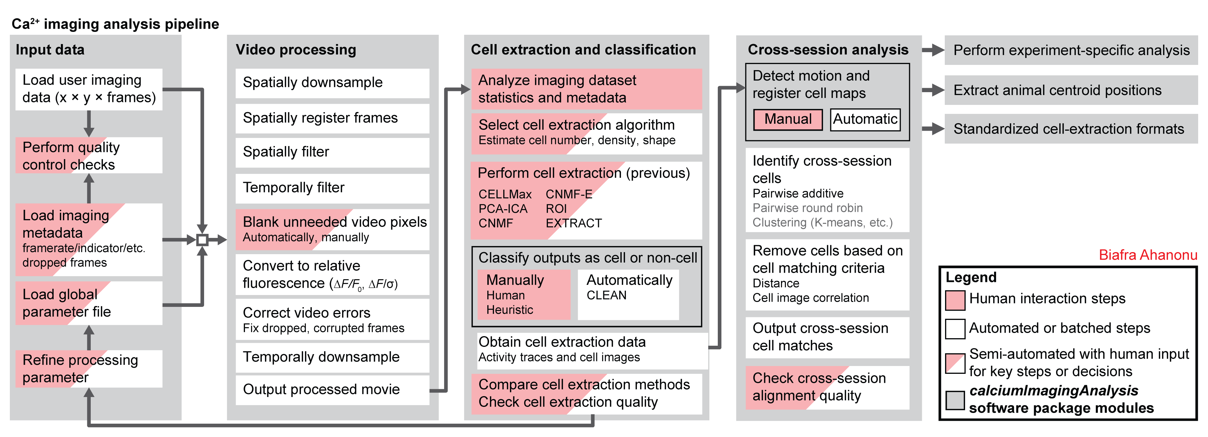
Processing calcium imaging data¶

The general pipeline for processing calcium imaging data is below. This repository includes code to do nearly every step.

Guides¶

Below are recordings for users who want to learn more about calcium imaging analysis.

Webinar¶

This webinar gives an overview of calcium imaging analysis (with a focus on CIAtah) along with tips for improving experiments and analysis: https://info.inscopix.com/inscopix-inspire-view-webinarbiafra-ahanonu-signal-in-the-noise-distinguishing-relevant-neural-activity-in-calcium-imaging.

Workshop tutorial¶

This recording gives an overview of setting up and using CIAtah: https://www.youtube.com/watch?v=I6abW3uuJJw.

Workflow¶

To start using the CIAtah software package, enter the following into the MATLAB command window.

% Loads all directories

loadBatchFxns;



% Loads the class into an object.

obj = ciatah;



% Open the class menu

obj % then hit enter, no semicolon!

% Alternatively

obj.runPipeline; % then hit enter!

The general order of functions that users should run is ([optional] are those not critical for most datasets):

• loadDependencies

  • If user is running CIAtah for the first time, this module has several options to download and load CNMF/CNMF-E code for cell extraction, Fiji for viewing/modifying videos (using Miji), and test data from a miniature microscope experiment.

• modelDownsampleRawMovies [optional]

  • If users have raw calcium imaging data that needs to be spatially downsampled, e.g. raw data from Inscopix nVista software.

• modelAddNewFolders

  • Users should always use this method first, used to add folders to the current class object.
  • For example, if users ran example_downloadTestData.m, then add the folder [githubRepoPath]\data\2014_04_01_p203_m19_check01_raw where githubRepoPath is the absolute path to the current CIAtah repository.

• viewMovie

  • Users should check that CIAtah loads their movies correctly and that Miji is working.
  • Users can view movies from disk, which allows checking of very large movies quickly.
  • Remember to check that Imaging movie regexp: (regular expression class uses to find user movies within given folders) setting matches name of movies currently in repository.

• viewMovieRegistrationTest [optional]

  • Users can check different spatial filtering and registration settings.
  • tregRunX folders (where X is a number) contain details of each run setting. Delete from analysis folder if don't need outputs later.
  • Remember to adjust contrast in resulting montage movies since different filtering will change the absolute pixel values.

• modelPreprocessMovie

  • Main processing method for CIAtah. Performs motion correction, spatial filtering, cropping, down-sampling, and relative fluorescence calculations. If using Inscopix nVista 1.0 or 2.0, also will correct for dropped frames.

• modelModifyMovies

  • GUI that allows users to remove movie regions not relevant to cell extraction.

• modelExtractSignalsFromMovie

  • Performs cell extraction on processed movies. Currently supports PCA-ICA, CNMF, CNMF-e, ROI, and EXTRACT. Support for CELLMax will be enabled in the public repository upon release.

• modelVarsFromFiles

  • Run after modelExtractSignalsFromMovie to load cell image and trace information into the current class object.

• viewCellExtractionOnMovie [optional]

  • This function overlays the cell extraction outputs on snippets of the processed video, allowing users to check that cell extraction correctly identified all the cells.

• computeManualSortSignals

  • A GUI to allow users to classify cells and not cells in cell extraction outputs.

• modelModifyRegionAnalysis [optional]

  • Users are able to select specific cells from cell extraction manual sorting to include in further analyses.

• computeMatchObjBtwnTrials

  • Method to register cells across imaging sessions. Also includes visual check GUI in viewMatchObjBtwnSessions method.
  • Note: it is heavily advised that throughout a particular animal's imaging sessions, that you keep the acquisition frame dimensions identical. This makes cross-session registration easier. Else you will have to crop all sessions for that animal to the same size ensuring that the area of interest is present in each.

  Detailed CIAtah processing pipeline¶

The following detailed pipeline assumes you have started a CIAtah object using the below command:

obj = ciatah;

Spatially downsample raw movies or convert to HDF5 with modelDownsampleRawMovies¶

Users have the ability to spatially downsample raw movies, often necessary to denoise the data, save storage space, and improve runtimes of later processing steps. For most data, users can downsample 2 or 4 times in each spatial dimension while still retaining sufficient pixels per cell to facilitate cell-extraction.

To run, either select modelDownsampleRawMovies in the GUI menu or type the below command after initializing a CIAtah obj.

obj.modelDownsampleRawMovies;

This will pop-up the following screen. Users can

• input several folders where ISXD files are by separating each folder path with a comma (Folder(s) where raw HDF5s are located),

• specify a common root folder to save files to (Folder to save downsampled HDF5s to:),

• and input a root directory that contains the sub-folders with the raw data (Decompression source root folder(s)).

The function will automatically put each file in its corresponding folder, make sure folder names are unique (this should be done anyways for data analysis reasons).

Converting Inscopix ISXD files to HDF5¶

To convert from Inscopix ISXD file format (output by nVista v3+ and nVoke) to HDF5 run modelDownsampleRawMovies without changing the regular expression or make sure it looks for .*.isxd or similar. Users will need the latest version of the Inscopix Data Processing Software as these functions take advantage of their API. If CIAtah cannot automatically find the API, it will ask the user to direct it to the root location of the Inscopix Data Processing Software (see below).

Check movie registration before pre-processing with viewMovieRegistrationTest¶

Users should spatially filter one-photon or other data with background noise (e.g. neuropil). To get a feel for how the different spatial filtering affects SNR/movie data before running the full processing pipeline, run viewMovieRegistrationTest module. Then select either matlab divide by lowpass before registering or matlab bandpass before registering then change filterBeforeRegFreqLow and filterBeforeRegFreqHigh settings, see below.

Within each folder will be a sub-folder called preprocRunTest inside of which is a series of sub-folders called preprocRun## that will contain a file called settings.mat that can be loaded into modelPreprocessMovie so the same settings that worked during the test can be used during the actual pre-processing run.

• You'll get an output like the below:

  • A: The top left is without any filtering while the other 3 are with different bandpass filtering options.
  • B: Cell ΔF/F intensity profile from the raw movie. Obtain by selecting Analyze->Plot profile from Fiji menu after selecting a square segment running through a cell.
  • C: Same cell ΔF/F intensity profile from the bottom/left movie (note the y-axis is the same as above). Obtained in same manner as B.

Preprocessing calcium imaging movies with modelPreprocessMovie¶

After users instantiate an object of the CIAtah class and enter a folder, they can start preprocessing of their calcium imaging data with modelPreprocessMovie.

• See below for a series of windows to get started, the options for motion correction, cropping unneeded regions, Δ_F/F_, and temporal downsampling were selected for use in the study associated with this repository.

• If users have not specified the path to Miji, a window appears asking them to select the path to Miji's scripts folder.

• If users are using the test dataset, it is recommended that they do not use temporal downsampling.

• Vertical and horizontal stripes in movies (e.g. CMOS camera artifacts) can be removed via stripeRemoval step. Remember to select correct stripOrientationRemove,stripSize, and stripfreqLowExclude options in the preprocessing options menu.

Next the user is presented with a series of options for motion correction, image registration, and cropping.:

• The options highlighted in green are those that should be considered by users.

• Users can over their mouse over each option to get tips on what they mean.

• In particular, make sure that inputDatasetName is correct for HDF5 files and that fileFilterRegexp matches the form of the calcium imaging movie files to be analyzed.

• After this, the user is asked to let the algorithm know how many frames of the movie to analyze (defaults to all frames).

• Then the user is asked to select a region to use for motion correction. In general, it is best to select areas with high contrast and static markers such as blood vessels. Stay away from the edge of the movie or areas outside the brain (e.g. the edge of microendoscope GRIN lens in one-photon miniature microscope movies).

Save/load preprocessing settings¶

Users can also enable saving and loading of previously selected pre-processing settings by changing the red option below.

Settings loaded from previous run (e.g. of modelPreprocessMovie) or file (e.g. from viewMovieRegistrationTest runs) are highlighted in orange. Settings that user has just changed are still highlighted in green.

The algorithm will then run all the requested preprocessing steps and presented the user with the option of viewing a slice of the processed file. Users have now completed pre-processing.

Manual movie cropping with modelModifyMovies¶

If users need to eliminate specific regions of their movie before running cell extraction, that option is provided. Users select a region using an ImageJ interface and select done when they want to move onto the next movie or start the cropping. Movies have NaNs or 0s added in the cropped region rather than changing the dimensions of the movie.

Extracting cells with modelExtractSignalsFromMovie¶

Users can run PCA-ICA, EXTRACT, CNMF, CNMF-E, and ROI cell extraction by following the below set of option screens. Details on running the new Schnitzer lab cell-extraction methods (e.g. CELLMax) will be added here after they are released.

We normally estimate the number of PCs and ICs on the high end, manually sort to get an estimate of the number of cells, then run PCA-ICA again with IC 1.5-3x the number of cells and PCs 1-1.5x number of ICs.

To run CNMF or CNMF-E, run loadDependencies module (e.g. obj.loadDependencies) after CIAtah class is loaded. CVX (a CNMF dependency) will also be downloaded and cvx_setup run to automatically set it up.

The resulting output (on Figure 45+) at the end should look something like:

Loading cell-extraction output data for custom scripts¶

Users can load outputs from cell extraction using the below command. This will then allow users to use the images and activity traces for downstream analysis as needed.

[inputImages,inputSignals,infoStruct,algorithmStr,inputSignals2] = ciapkg.io.loadSignalExtraction('pathToFile');

Note, the outputs correspond to the below:

• inputImages - 3D or 4D matrix containing cells and their spatial information, format: [x y nCells].

• inputSignals - 2D matrix containing activity traces in [nCells nFrames] format.

• infoStruct - contains information about the file, e.g. the 'description' property that can contain information about the algorithm.

• algorithmStr - String of the algorithm name.

• inputSignals2 - same as inputSignals but for secondary traces an algorithm outputs.

Loading cell-extraction output data with modelVarsFromFiles¶

In general, after running cell-extraction (modelExtractSignalsFromMovie) on a dataset, run the modelVarsFromFiles module. This allows CIAtah to load/pre-load information about that cell-extraction run.

If you had to restart MATLAB or are just loading CIAtah fresh but have previously run cell extraction, run this method before doing anything else with that cell-extraction data.

A menu will pop-up like below when modelVarsFromFiles is loaded, you can normally just leave the defaults as is.

Validating cell extraction with viewCellExtractionOnMovie¶

After users have run cell extraction, they should check that cells are not being missed during the process. Running the method viewCellExtractionOnMovie will create a movie with outlines of cell extraction outputs overlaid on the movie.

Below is an example, with black outlines indicating location of cell extraction outputs. If users see active cells (red flashes) that are not outlined, that indicates either exclusion or other parameters should be altered in the previous modelExtractSignalsFromMovie cell extraction step.

Sorting cell extraction outputs with computeManualSortSignals¶

CIAtah cell sorting GUI

Outputs from most common cell-extraction algorithms like PCA-ICA, CNMF, etc. contain signal sources that are not cells and thus must be manually removed from the output. The repository contains a GUI for sorting cells from not cells. GUI also contains a shortcut menu that users can access by right-clicking or selecting the top-left menu.

Below users can see a list of options that are given before running the code, those highlighted in green

GUI usage on large imaging datasets¶

• To manually sort on large movies that will not fit into RAM, select the below options (highlighted in green). This will load only chunks of the movie asynchronously into the GUI as you sort cell extraction outputs.

Cell sorting from the command line with signalSorter¶

Usage instructions below for signalSorter, e.g. if not using the CIAtah GUI.

Main inputs

• inputImages - [x y N] matrix where N = number of images, x/y are dimensions.

• inputSignals - [N frames] double matrix where N = number of signals (traces).

• inputMovie - [x y frames] matrix

Main outputs

• choices - [N 1] vector of 1 = cell, 0 = not a cell

• inputImagesSorted - [x y N] filtered by choices

• inputSignalsSorted - [N frames] filtered by choice

iopts.inputMovie = inputMovie; % movie associated with traces

iopts.valid = 'neutralStart'; % all choices start out gray or neutral to not bias user

iopts.cropSizeLength = 20; % region, in px, around a signal source for transient cut movies (subplot 2)

iopts.cropSize = 20; % see above

iopts.medianFilterTrace = 0; % whether to subtract a rolling median from trace

iopts.subtractMean = 0; % whether to subtract the trace mean

iopts.movieMin = -0.01; % helps set contrast for subplot 2, preset movie min here or it is calculated

iopts.movieMax = 0.05; % helps set contrast for subplot 2, preset movie max here or it is calculated

iopts.backgroundGood = [208,229,180]/255;

iopts.backgroundBad = [244,166,166]/255;

iopts.backgroundNeutral = repmat(230,[1 3])/255;

[inputImagesSorted, inputSignalsSorted, choices] = signalSorter(inputImages, inputSignals, 'options',iopts);

Examples of the interface on two different datasets:

BLA one-photon imaging data signal sorting GUI¶

mPFC one-photon imaging data signal sorting GUI (from example_downloadTestData.m)¶

Context menu¶

Removing cells not within brain region with modelModifyRegionAnalysis¶

If the imaging field-of-view includes cells from other brain regions, they can be removed using modelModifyRegionAnalysis

Cross-session cell alignment with computeMatchObjBtwnTrials¶

This step allows users to align cells across imaging sessions (e.g. those taken on different days). See the Cross session cell alignment wiki page for more details and notes on cross-session alignment.

• Users run computeMatchObjBtwnTrials to do cross-day alignment (first row in pictures below).

• Users then run viewMatchObjBtwnSessions to get a sense for how well the alignment ran.

• computeCellDistances and computeCrossDayDistancesAlignment allow users to compute the within session pairwise Euclidean centroid distance for all cells and the cross-session pairwise distance for all global matched cells, respectively.

Users can then get the matrix that gives the session IDs

% Global IDs is a matrix of [globalID sessionID]

% Each (globalID, sessionID) pair gives the within session ID for that particular global ID

globalIDs = alignmentStruct.globalIDs;

View cross-session cell alignment with viewMatchObjBtwnSessions¶

To evaluate how well cross-session alignment works, computeMatchObjBtwnTrials will automatically run viewMatchObjBtwnSessions at the end, but users can also run it separately after alignment. The left are raw dorsal striatum cell maps from a single animal. The right shows after cross-session alignment; color is used to indicate a global ID cell (e.g. the same cell matched across multiple days). Thus, same color cell = same cell across sessions.

Save cross-session cell alignment with modelSaveMatchObjBtwnTrials¶

Users can save out the alignment structure by running modelSaveMatchObjBtwnTrials. This will allow users to select a folder where CIAtah will save a MAT-file with the alignment structure information for each animal.

ImageJ+MATLAB based mouse location tracking¶

Functions needed (have entire CIAtah loaded anyways):

• mm_tracking.ijm is the tracking function for use in ImageJ, place in

plugins folder. If already had CIAtah download Fiji, place in the _external_programs/[Fiji directory]/Fiji.app/plugins folder.

• removeIncorrectObjs.m is a function to clean-up the ImageJ output.

• createTrackingOverlayVideo is a way to check the output from the

tracking by overlaying mouse tracker onto the video.

Instructions for ImageJ and Matlab¶

Example screen after running mm_tracking within ImageJ, click to expand.

After the above screen, there will be multiple other screens culminating in one where a threshold is chosen that is used to remove non-animal pixels from analysis. The threshold matters quite a bit and the script ignores anything that isn't red (i.e. larger than threshold) OR not within the range specified by the parameters below.

The script opens the AVI as a virtual stack and asks for the threshold is so that I can quickly scan through the entire movie to make sure the set threshold works even with slight/major changes in illumination, e.g. the below threshold will work across many frames

If the threshold is set to low, certain frames will not have the animal detected, e.g. if the lighting changes.

Once ImageJ is finished, within Matlab run the following code (cleans up the ImageJ tracking by removing small objects and adding NaNs for missing frames along with making a movie to check output). Modify to point toward paths specific for your data.

% CSV file from imageJ and AVI movie path used in ImageJ

moviePath = 'PATH_TO_AVI_USED_IN_IMAEJ';

csvPath = 'PATH_TO_CSV_OUTPUT_BY_IMAGEJ';

% clean up tracking

[trackingTableFilteredCell] = removeIncorrectObjs(csvPath,'inputMovie',{moviePath});

% make tracking video

% frames to use as example check

nFrames=1500:2500;

inputMovie = loadMovieList(moviePath,'frameList',nFrames);

[inputTrackingVideo] = createTrackingOverlayVideo(inputMovie,movmean(trackingTableFilteredCell.XM(nFrames),5),movmean(trackingTableFilteredCell.YM(nFrames),5));

playMovie(inputTrackingVideo);

Example output from 2017_09_11_p540_m381_openfield01_091112017¶

Using createTrackingOverlayVideo to verify tracking matches animal position on a per frame basis.

—API—

¶

Example CIAtah pipeline via the command line.¶

Below is an example CIAtah pipeline using the command line for those that do not want to use the class or want to create their own custom batch analyses. It assumes you have already run example_downloadTestData to download the example test data and have MATLAB path set to the CIAtah root directory.

Can also access the pipeline by typing edit ciapkg.demo.cmdLinePipeline into the MATLAB command window or run by typing in ciapkg.demo.cmdLinePipeline;.

Setup¶

% Running CIAtah from MATLAB command line/window



guiEnabled = 1;

saveAnalysis = 1;

inputDatasetName = '/1';

rawFileRegexp = 'concat';



% Setup folder paths

analysisFolderPath = [ciapkg.getDir() filesep 'data' filesep '2014_04_01_p203_m19_check01'];

[~,folderName,~] = fileparts(analysisFolderPath);

% Setup NWB folder paths

nwbFilePath = [analysisFolderPath filesep 'nwbFiles' filesep folderName];

nwbFileFolderPath = [analysisFolderPath filesep 'nwbFiles'];



% Load CIAtah functions

loadBatchFxns();

%% Download test data, only a single session

ciapkg.api.example_downloadTestData('downloadExtraFiles',0);

%% Load movie to analyze

inputMoviePath = ciapkg.api.getFileList(analysisFolderPath,rawFileRegexp,'sortMethod','natural');

% inputMoviePath = [analysisFolderPath filesep 'concat_recording_20140401_180333.h5'];

inputMovie = ciapkg.api.loadMovieList(inputMoviePath,'inputDatasetName',inputDatasetName);

Visualize movie¶

%% Visualize slice of the movie

ciapkg.api.playMovie(inputMovie(:,:,1:500),'extraTitleText','Raw movie');

% Alternatively, visualize by entering the file path

ciapkg.api.playMovie(inputMoviePath,'extraTitleText','Raw movie directly from file');

Downsample movie¶

%% Downsample input movie if need to

inputMovieD = ciapkg.api.downsampleMovie(inputMovie,'downsampleDimension','space','downsampleFactor',4);

ciapkg.api.playMovie(inputMovie,'extraMovie',inputMovieD,'extraTitleText','Raw movie vs. down-sampled movie');



% Alternatively, if you have Inscopix ISXD files, downsample by reading segments from disk using.

moviePath = 'PATH_TO_ISXD';

opts.maxChunkSize = 5000; % Max chunk size in Mb to load into RAM.

opts.downsampleFactor = 4; % How much to downsample original movie, set to 1 for no downsampling.

ciapkg.api.convertInscopixIsxdToHdf5(moviePath,'options',opts);

Remove stripe artifacts (e.g. from camera) from movie¶

%% Remove stripes from movie if needed

% Show full filter sequence for one frame

sopts.stripOrientation = 'both';

sopts.meanFilterSize = 1;

sopts.freqLowExclude = 10;

sopts.bandpassType = 'highpass';

ciapkg.api.removeStripsFromMovie(inputMovie(:,:,1),'options',sopts,'showImages',1);

% Run on the entire movie

ciapkg.api.removeStripsFromMovie(inputMovie,'options',sopts);

Detrend movie if needed (default linear trend), e.g. to compensate for bleaching over time.¶

%% Detrend movie

inputMovie = ciapkg.api.normalizeMovie(inputMovie,'normalizationType','detrend','detrendDegree',1);

Run motion correction¶

%% Get coordinates to crop from the user separately or set automatically

if guiEnabled==1

    [cropCoords] = ciapkg.api.getCropCoords(squeeze(inputMovie(:,:,1)));

    toptions.cropCoords = cropCoords;

    % Or have turboreg function itself directly ask the user for manual area from which to obtain correction coordinates

    % toptions.cropCoords = 'manual';

else

    toptions.cropCoords = [26 34 212 188];

end

%% Motion correction

% Or have turboreg run manual correction

toptions.cropCoords = 'manual';

toptions.turboregRotation = 0;

toptions.removeEdges = 1;

toptions.pxToCrop = 10;

% Pre-motion correction

    toptions.complementMatrix = 1;

    toptions.meanSubtract = 1;

    toptions.meanSubtractNormalize = 1;

    toptions.normalizeType = 'matlabDisk';

% Spatial filter

    toptions.normalizeBeforeRegister = 'divideByLowpass';

    toptions.freqLow = 0;

    toptions.freqHigh = 7;

[inputMovie2, ~] = ciapkg.api.turboregMovie(inputMovie,'options',toptions);

%% Compare raw and motion corrected movies

ciapkg.api.playMovie(inputMovie,'extraMovie',inputMovie2);

Convert movie to units of relative fluorescence¶

%% Run dF/F

inputMovie3 = ciapkg.api.dfofMovie(single(inputMovie2),'dfofType','dfof');

Downsample movie¶

%% Run temporal downsampling

inputMovie3 = ciapkg.api.downsampleMovie(inputMovie3,'downsampleDimension','time','downsampleFactor',4);

%% Final check of movie before cell extraction

ciapkg.api.playMovie(inputMovie3);

Run PCA-ICA¶

%% Run PCA-ICA cell extraction. CNMF-e, CNMF, ROI, and other cell-extraction algorithms are also available.

nPCs = 300;

nICs = 225;

pcaicaStruct = ciapkg.signal_extraction.runPcaIca(inputMovie3,nPCs,nICs,'version',2,'output_units','fl','mu',0.1,'term_tol',5e-6,'max_iter',1e3);

%% Save outputs to NWB format

if saveAnalysis==1

    ciapkg.api.saveNeurodataWithoutBorders(pcaicaStruct.IcaFilters,{pcaicaStruct.IcaTraces},'pcaica',[nwbFilePath '_pcaicaAnalysis.nwb']);

end

Run CNMF or CNMF-e cell extraction.¶

%% Run CNMF or CNMF-e cell extraction

numExpectedComponents = 225;

cellWidth = 10;

cnmfOptions.otherCNMF.tau = cellWidth/2; % expected width of cells



% Run CNMF

[success] = ciapkg.api.cnmfVersionDirLoad('current');

[cnmfAnalysisOutput] = ciapkg.api.computeCnmfSignalExtractionClass(inputMovie3,numExpectedComponents,'options',cnmfOptions);



% Run CNMF-e

[success] = ciapkg.api.cnmfVersionDirLoad('cnmfe');

cnmfeOptions.gSiz = cellWidth;

cnmfeOptions.gSig = ceil(cellWidth/4);

[cnmfeAnalysisOutput] = ciapkg.api.computeCnmfeSignalExtraction_batch(outputMoviePath,'options',cnmfeOptions);



% Save outputs to NWB format

if saveAnalysis==1

    % Save CNMF

    ciapkg.api.saveNeurodataWithoutBorders(cnmfAnalysisOutput.extractedImages,{cnmfAnalysisOutput.extractedSignals,cnmfAnalysisOutput.extractedSignalsEst},'cnmf',[nwbFilePath '_cnmf.nwb']);



    % Save CNMF-E

    ciapkg.api.saveNeurodataWithoutBorders(cnmfeAnalysisOutput.extractedImages,{cnmfeAnalysisOutput.extractedSignals,cnmfeAnalysisOutput.extractedSignalsEst},'cnmfe',[nwbFilePath '_cnmfe.nwb']);

end



[success] = ciapkg.api.cnmfVersionDirLoad('none');

Run EXTRACT cell extraction.¶

%% Run EXTRACT cell extraction. Check each function with "edit" for options.

% Load default configuration

ciapkg.loadBatchFxns('loadEverything');

extractConfig = get_defaults([]);



% See https://github.com/schnitzer-lab/EXTRACT-public#configurations.

cellWidth = 10;

extractConfig.avg_cell_radius = cellWidth;

extractConfig.num_partitions_x = 2;

extractConfig.num_partitions_y = 2;

extractConfig.use_sparse_arrays = 0;



outStruct = extractor(inputMovie3,extractConfig);



% Grab outputs and put into standard format

extractAnalysisOutput.filters = outStruct.spatial_weights;

% permute so it is [nCells frames]

extractAnalysisOutput.traces = permute(outStruct.temporal_weights, [2 1]);



% Other run information if saving as a MAT-file.

extractAnalysisOutput.info = outStruct.info;

extractAnalysisOutput.config = outStruct.config;

extractAnalysisOutput.info = outStruct.info;

extractAnalysisOutput.userInputConfig = extractConfig;

extractAnalysisOutput.opts = outStruct.config;



% Save outputs to NWB format

if saveAnalysis==1

    ciapkg.api.saveNeurodataWithoutBorders(extractAnalysisOutput.filters,{extractAnalysisOutput.traces},'extract',[nwbFilePath '_extract.nwb']);

end



% Remove EXTRACT from the path.

ciapkg.loadBatchFxns();

Manual sort output cells¶

%% Run signal sorting using matrix inputs

[outImages, outSignals, choices] = ciapkg.api.signalSorter(IcaFilters,IcaTraces,'inputMovie',inputMovie3);

Run signal sorting using NWB¶

%% Run signal sorting using NWB

[outImages, outSignals, choices] = ciapkg.api.signalSorter([nwbFilePath '_pcaicaAnalysis.nwb'],[],'inputMovie',inputMovie3);

%% Plot results of sorting

figure;

subplot(1,2,1);imagesc(max(IcaFilters,[],3));axis equal tight; title('Raw filters')

subplot(1,2,2);imagesc(max(outImages,[],3));axis equal tight; title('Sorted filters')

Run signal sorting using multiple NWB files from cell extraction.¶

% Run signal sorting using NWB files from cell extraction.

if saveAnalysis==1&guiEnabled==1

    disp(repmat('=',1,21));disp('Running signalSorter using NWB file input.')

    nwbFileList = ciapkg.api.getFileList(nwbFileFolderPath,'.nwb');

    if ~isempty(nwbFileList)

        nFiles = length(nwbFileList);

        outImages = {};

        outSignals = {};

        choices = {};

        for fileNo = 1:nFiles

            [outImages{fileNo}, outSignals{fileNo}, choices{fileNo}] = ciapkg.api.signalSorter(nwbFileList{fileNo},[],'inputMovie',inputMovie3);

        end



        % Plot results of sorting

        for fileNo = 1:nFiles

            try

                [inputImagesTmp,inputSignalsTmp,infoStructTmp,algorithmStrTmp,inputSignals2Tmp] = ciapkg.io.loadSignalExtraction(nwbFileList{fileNo});

                figure;

                subplot(1,2,1); 

                    imagesc(max(inputImagesTmp,[],3));

                    axis equal tight; 

                    title([algorithmStrTmp ' | Raw filters'])

                subplot(1,2,2); 

                    imagesc(max(outImages{fileNo},[],3));

                    axis equal tight; 

                    title('Sorted filters')

            catch err

                disp(repmat('@',1,7))

                disp(getReport(err,'extended','hyperlinks','on'));

                disp(repmat('@',1,7))

            end

        end

    end

end

Overlay cells on movies as sanity check¶

%% Create an overlay of extraction outputs on the movie and signal-based movie

[inputMovieO] = ciapkg.api.createImageOutlineOnMovie(inputMovie3,IcaFilters,'dilateOutlinesFactor',0);

[signalMovie] = ciapkg.api.createSignalBasedMovie(IcaTraces,IcaFilters,'signalType','peak');

%% Play all three movies

% Normalize all the movies

movieM = cellfun(@(x) ciapkg.api.normalizeVector(x,'normRange','zeroToOne'),{inputMovie3,inputMovieO,signalMovie},'UniformOutput',false);

ciapkg.api.playMovie(cat(2,movieM{:}));

Batch process example movies and perform cross-session cell alignment¶

%% Run pre-processing on 3 batch movies then do cross-session alignment

batchMovieList = {...

[ciapkg.getDir() filesep 'data' filesep 'batch' filesep '2014_08_05_p104_m19_PAV08'],...

[ciapkg.getDir() filesep 'data' filesep 'batch' filesep '2014_08_06_p104_m19_PAV09'],...

[ciapkg.getDir() filesep 'data' filesep 'batch' filesep '2014_08_07_p104_m19_PAV10']...

};

% USER INTERFACE Get the motion correction crop coordinates

cropCoordsCell = {};

nFolders = length(batchMovieList);

for folderNo = 1:nFolders

    analysisFolderPath = batchMovieList{folderNo};

    inputMoviePath = ciapkg.api.getFileList(analysisFolderPath,rawFileRegexp,'sortMethod','natural');

    % inputMoviePath = [analysisFolderPath filesep 'concat_recording_20140401_180333.h5'];

    inputMovie = ciapkg.api.loadMovieList(inputMoviePath,'inputDatasetName',inputDatasetName,'frameList',1:2);



    [cropCoords] = ciapkg.api.getCropCoords(squeeze(inputMovie(:,:,1)));

    % toptions.cropCoords = cropCoords;

    cropCoordsCell{folderNo} = cropCoords;

end

%% Run pre-processing on each of the movies.

procMovieCell = cell([1 nFolders]);

for folderNo = 1:nFolders

    inputMoviePath = ciapkg.api.getFileList(analysisFolderPath,rawFileRegexp,'sortMethod','natural');

    inputMovie = ciapkg.api.loadMovieList(inputMoviePath,'inputDatasetName',inputDatasetName,'frameList',[]);

    procOpts.motionCorrectionCropCoords = cropCoordsCell{folderNo};

    procOpts.dfofMovie = 1;

    procOpts.motionCorrectionFlag = 1;

    procOpts.normalizeMovieFlag = 1;

    procOpts.normalizeType = 'divideByLowpass';

    procOpts.freqLow = 0;

    procOpts.freqHigh = 7;

    procOpts.downsampleTimeFactor = 4;

    procMovieCell{folderNo} = ciapkg.demo.runPreprocessing(inputMovie,'options',procOpts);

end

disp('Done with pre-processing!')

%% Run cell-extraction on the movies

pcaicaStructCell = cell([1 nFolders]);

nPCs = 300;

nICs = 225;

for folderNo = 1:nFolders

    inputMoviePath = ciapkg.api.getFileList(analysisFolderPath,rawFileRegexp,'sortMethod','natural');

    pcaicaStruct{folderNo} = ciapkg.signal_extraction.runPcaIca(procMovieCell{folderNo},nPCs,nICs,'version',2,'outputUnits','fl','mu',0.1,'term_tol',5e-6,'max_iter',1e3);

end

disp('Done with PCA-ICA analysis pre-processing!')

%% Run cross-session alignment of cells

% Create input images, cell array of [x y nCells] matrices

inputImages = cellfun(@(x) x.IcaFilters,pcaicaStruct,'UniformOutput',false);



% options to change

opts.maxDistance = 5; % distance in pixels between centroids for them to be grouped

opts.trialToAlign = 1; % which session to start alignment on

opts.nCorrections = 1; %number of rounds to register session cell maps.

opts.RegisTypeFinal = 2; % 3 = rotation/translation and iso scaling; 2 = rotation/translation, no iso scaling



% Run alignment code

[alignmentStruct] = ciapkg.api.matchObjBtwnTrials(inputImages,'options',opts);



% Global IDs is a matrix of [globalID sessionID]

% Each (globalID, sessionID) pair gives the within session ID for that particular global ID

globalIDs = alignmentStruct.globalIDs;



% View the cross-session matched cells, saved to `private\_tmpFiles` sub-folder.

[success] = ciapkg.api.createMatchObjBtwnTrialsMaps(inputImages,alignmentStruct);

%% Display cross-session matching movies

disp('Playing movie frames')

crossSessionMovie1 = [ciapkg.getDir filesep 'private' filesep '_tmpFiles' filesep 'matchObjColorMap50percentMatchedSession_matchedCells.avi'];

crossSessionMovie2 = [ciapkg.getDir filesep 'private' filesep '_tmpFiles' filesep 'matchObjColorMapAllMatchedSession_matchedCells.avi'];

ciapkg.api.playMovie(crossSessionMovie1,'extraMovie',crossSessionMovie2,'rgbDisplay',1);

CIAtah functions within {{ code.package }} sub-package.¶

CIAtah contains many functions for imaging analysis, from processing videos to wrappers for running cell extraction algorithms and GUIs for visualizing movies and evaluating cell extraction outputs. Several are detailed below. For each users can visualize options with help FUN or edit FUN. If attempting to load a non-package function (e.g. it does not start with {{ code.package }}), then append {{ code.package }}.api., e.g. playMovie would become {{ code.package }}.api.playMovie. Alternatively, load all the functions into the workspace with import ciapkg.api.*.

This page will be further updated with information soon.

Visualizing movies¶

playMovie

ciapkg.io.loadMovie or loadMovieList

createImageOutlineOnMovie

createSignalBasedMovie

ciapkg.io.readFrame

Get movie information¶

ciapkg.io.getMovieInfo

Sorting cells¶

signalSorter

Pre-processing¶

ciapkg.demo.runPreprocessing

downsampleHdf5Movie

removeStripsFromMovie

turboregMovie

dfofMovie

downsampleMovie

normalizeMovie

Cell extraction¶

• PCA-ICA - ciapkg.signal_extraction.runPcaIca.

Cross-session alignment¶

matchObjBtwnTrials

createMatchObjBtwnTrialsMaps

—Help—

¶

Common issues and fixes¶

Page outlines some common issues and fixes to them that may be encountered while using CIAtah. These are mostly due to quirks specific to MATLAB, Fiji, or the computing environment CIAtah is used on.

Contents¶

• PCA-ICA, CNMF-E, or other cell extraction algorithm's don't produce sensible output.

• Out of memory using Miji

• Selecting scripts folder in Fiji.app on Mac OS X

• Fiji won't start using Miji or MIJ.start

• downloadCnmfGithubRepositories.m not downloading correctly

• modelPreprocessMovie analysis options list not showing

• Miji not loading correctly

• viewMovie or other functions where movies need to be loaded end without executing

• Contrast is low on cell transient ΔF/F movies using computeManualSortSignals

• Traces in computeManualSortSignals GUI are flat.

  • Can't see transients.
  • Change the min/max.
  • Can now see transients.

• Blank frames or entire frames have baseline shifted after motion correction in modelPreprocessMovie

• File or folder dialog box with no instructions

Error opening AVI or other files due to codec issues¶

If run into issues opening certain AVI files (e.g. due to codec issues) with CIAtah/MATLAB:

Error using VideoReader/initReader (line 734)

Unable to determine the required codec.



Error in audiovideo.internal.IVideoReader (line 136)

            initReader(obj, fileName, currentTime);



Error in VideoReader (line 104)

            obj@audiovideo.internal.IVideoReader(varargin{:});

, install K-Lite Codec Pack (https://codecguide.com/download_kl.htm) or similar for added support.

PCA-ICA, CNMF-E, or other cell extraction algorithm's don't produce sensible output.¶

• When running modelPreprocessMovie a dialog box appears showing the available analysis steps. Certain combinations of these steps make sense while others should be avoided.

• For example, normally users want turboreg->crop->dfof->downsampleTime.

• An invalid input would be turboreg->crop->dfof->dfstd->downsampleTime. Since calculating the dF/F then dF/std is problematic.

• For two photon data, it is sometimes desired to have medianFilter->turboreg->crop->dfstd (or dfof)->downsampleTime.

• In general, fft_highpass and fft_lowpass should be avoided since they are meant to be run on stand-alone movies for specific purposes rather than included in the general pipeline.

• Remember at the options screen (see below) to select a spatial filtering there under the option filterBeforeRegister instead of selecting the spatialFilter option before the turboreg option in the analysis steps screen.

Out of memory using Miji¶

• If you get a java.lang.OutOfMemoryError: GC overhead limit exceeded style error (see below code) when trying to open a movie with Miji, make sure that you initialize MATLAB in the CIAtah path or place the java.opts file in your MATLAB start-up folder.

java.lang.OutOfMemoryError: GC overhead limit exceeded

    at java.lang.AbstractStringBuilder.<init>(Unknown Source)

    at java.lang.StringBuilder.<init>(Unknown Source)

• On Windows, you can change the start-up folder as below or in general see https://www.mathworks.com/help/matlab/matlab_env/matlab-startup-folder.html.

• java.opts increases the amount of memory allocated so that Java doesn't run out when using Miji to load movies. To change the amount of memory allocated (CIAtah sets to 7 Gb by default), change the below to a higher or lower number, e.g. 9 Gb would be -Xmx9000m.

-Xmx7000m

Selecting scripts folder in Fiji.app on Mac OS X¶

Navigate to the applications folder and select Fiji.app and Show Package Contents.

Then navigate to /Fiji.app/scripts and select Miji.m then Get Info. Select and copy the path as below.

When Matlab ask for the Fiji path, press command + shift + G in the dialog box to enter the full path manually, press enter, then select open.

Fiji won't start using Miji or MIJ.start¶

• If calling Miji or MIJ.start does not lead to a Fiji GUI appearing (e.g. the below output is seen in the command window), this is likely because the last Fiji/ImageJ instance was closed improperly (e.g. by closing ImageJ with File->Quit or pressing the close button instead of MIJ.exit in the Matlab command window), leading to a headless Fiji that cannot be properly closed by Miji/Matlab.

--------------------------------------------------------------

Status> ImageJ is already started.

--------------------------------------------------------------

If this occurs, run the following commands one at a time:

resetMiji

% An instance of Miji should appear.

currP=pwd;Miji;cd(currP);

MIJ.exit

downloadCnmfGithubRepositories.m not downloading correctly¶

• If when trying to download using downloadCnmfGithubRepositories.m the below error is encountered, try to run downloadCnmfGithubRepositories several more times as websave (MATLAB built-in function) sometimes momentarily does not obtain the correct write permissions and fails.

@@@@@@@

Error using websave (line 104)

Unable to open output file: 'signal_extraction\cnmfe.zip' for writing. Common reasons include that the file exists and does not have write permission or the folder does not have write permissions.

modelPreprocessMovie analysis options list not showing¶

• MATLAB changed uitables internal implementation, hence findjobj (File Exchange function) broke causing reorderableListbox (File Exchange function) to also break. An updated findjobj has been added to the CIAtah repository and this error (see below) should no longer occur.

Error in reorderableListbox (line 127)

jScrollPane = jScrollPane(1);

Miji not loading correctly¶

• The below error occurs when the wrong version of Fiji is downloaded. Please 2015 December 22 version download from https://imagej.net/Fiji/Downloads as that implementation of Miji.m appears to work correctly with MATLAB.

@@@@@@@

Error using javaObject

No class MIJ can be located on the Java class path

viewMovie or other functions where movies need to be loaded end without executing¶

• It is likely that the regular expression given to CIAtah does not match any of the files in the folder being analyzed.

• For example, in viewMovie, the below Image movie regexp setting should be changed to concat correspond to the demo raw imaging data's name.

Contrast is low on cell transient ΔF/F movies using computeManualSortSignals¶

• The contrast (e.g. min/max) are estimated automatically from movie data, but will not always be the optimal display for manual human sorting of data. To improve the contrast, press q while in the interface and adjust the min/max values until you are in a satisfactory range. See below.

Default contrast:

Contrast after user editing:

Traces in computeManualSortSignals GUI are flat.¶

• Likely this is due to one of the traces having values that are very high, throwing off the estimate used set the y-axis in the GUI (which is constant across all candidate cells). This can be changed by pressing w, see below.

Can't see transients.¶

Change the min/max.¶

Can now see transients.¶

Blank frames or entire frames have baseline shifted after motion correction in modelPreprocessMovie¶

• This normally occurs when transfturboreg is selected as the registrationFxn, in some Windows editions and OSX versions this leads to random baseline shifts. If this occurs change registrationFxn to imtransform. See below (green selected option).

File or folder dialog box with no instructions¶

• This is mainly on OS X, where in some versions the dialog boxes are not styled with title bars (see below). This is outside of MATLAB's control. If this occurs, check the command window as the instructions should also be provided there (e.g. with Dialog box: [TITLE] style text).

Inscopix¶

Documentation related to Inscopix-specific functions on the repository.

Visualizing ISXD files¶

ISXD files can be directly visualized from disk by running playMovie from MATLAB command line:

playMovie('path\to\youMovie.isxd');

Converting ISXD files to HDF5¶

To convert ISXD files to HDF5, see convertInscopixIsxdToHdf5 function in the inscopix folder or modelDownsampleRawMovies module in CIAtah.

Note: By default the Inscopix API gives out a frame full of 0s for dropped frames. So those 0s frames are maintained after converting/downsampling to HDF5 or you will also get a frame with 0s if you use loadMovieList to read frames that were dropped from isxd files. Adjust analysis accordingly.

To use this function call it as below:

moviePath = 'PATH_TO_ISXD';

opts.maxChunkSize = 5000; % Max chunk size in Mb to load into RAM.

opts.downsampleFactor = 4; % How much to downsample original movie, set to 1 for no downsampling.

convertInscopixIsxdToHdf5(moviePath,'options',opts);

If you want to save to a custom folder, use saveFolder input.

moviePath = 'PATH_TO_ISXD';

opts.maxChunkSize = 5000; % Max chunk size in Mb to load into RAM.

opts.downsampleFactor = 4; % How much to downsample original movie, set to 1 for no downsampling.

opts.saveFolder = 'ALT_FOLDER_PATH'; % Char: alternative file path

convertInscopixIsxdToHdf5(moviePath,'options',opts);

The same functionality can be achieved by loading a CIAtah module using the below commands. By default modelDownsampleRawMovies module will see .isxd files and call convertInscopixIsxdToHdf5. This can be done on multiple folders by separating them with commas in the modelDownsampleRawMovies menu.

obj = ciatah;

obj.modelDownsampleRawMovies;

Neurodata Without Borders (NWB)¶

NWB is a data standard

Some movies are larger than the available RAM on users analysis computer. Below are several ways that the underlying functions in CIAPKG can be used to analyze large movies.

https://neurodatawithoutborders.github.io/matnwb/tutorials/html/ophys.html

Saving NWB¶

% Full path to the movie

saveNeurodataWithoutBorders(cellExtractionImages,{cellExtractionSignals},cellExtractionAlgorithm,nwbFilePath);

Where cellExtractionAlgorithm is the algorithm used, consisting of:

Loading NWB¶

% Full path to the movie

[inputImages,inputTraces,infoStruct, algorithmStr] = loadNeurodataWithoutBorders(nwbFilePath);

Outputs mean:

• inputImages - 3D or 4D matrix containing cells and their spatial information.

• inputTraces - 2D matrix containing trace outputs.

• infoStruct - contains information about the file, e.g. the 'description' property that can contain information about the algorithm.

• algorithmStr - String of the algorithm name.

Using NWB with signalSorter¶

For manual sorting, users can directly input path to NWB file as below:

[outImages, outSignals, choices] = signalSorter('pcaica.nwb',[],'inputMovie',inputMoviePath);

Interpreting displayed movies¶

It may appear at times that CIAtah has introduced noise into movies after processing. However, normally that noise is already there in the movie. In the case of one-photon miniature microscope movies that noise is often small relative to the baseline background fluorescence, hence not noticeable. However, after dF/F0 or spatial filtering users will be able to see the noise more easily as it will have a relatively greater magnitude compared to the signal now present in the movie.

Further, in many cases the contrast is automatically adjusted in CIAtah GUIs to boost likelihood users will see cells and other biologically relevant features (even though underlying matrix values are not changed), which can sometimes lead to the perception that noise is being added depending on viewing raw vs. dF/F0 or other preprocessed movies.

Example¶

For example of what this looks like, take one of the example movies in the CIAtah repository: 2014_04_01_p203_m19_check01.

Raw movie¶

A frame from the raw movie looks like:

Applying a simple bandpass or highpass filter (to remove the low frequency background) leads to the below (keeping contrast/brightness the same as the raw movie image):

However, if we adjust the contrast, we can now see some of the noise present in the higher frequency components of the raw movie that was otherwise obscured or would be hard to see in the raw movie with the high baseline present:

dF/F0¶

Now compare to dF/F0 of that same raw movie without any motion correction, etc. we see the below:

However, if you adjust the contrast, you get the below image, where the noise is much more pronounced:

Imaging analysis methods and code¶

Outline of outside code, software packages, or techniques relevant to calcium imaging analysis. Also includes links to papers or GitHub code repositories.

Find an overview of calcium imaging analysis methods at https://bahanonu.com/brain/#c20181209. Or see below.

Image Registration¶

• Turboreg

  • http://bigwww.epfl.ch/thevenaz/turboreg/

• NoRMCorre

  • https://github.com/simonsfoundation/NoRMCorre

• moco

  • https://github.com/NTCColumbia/moco

Cross-day alignment¶

• CellReg (Ziv lab)

  • https://github.com/zivlab/CellReg/issues/1

Cell segmentation (static image)¶

• NeuroSeg: automated cell detection and segmentation for in vivo two-photon Ca2+ imaging data

  • https://link.springer.com/article/10.1007/s00429-017-1545-5
  • https://github.com/baidatong/NeuroSeg

Cell extraction (dynamic movie)¶

• PCA-ICA (Schnitzer)

  • https://www.ncbi.nlm.nih.gov/pmc/articles/PMC3282191/
  • https://github.com/schnitzer-lab/miniscope_analysis/tree/master/signal_extraction/pca_ica

• CELLMax (Schnitzer)

  • https://github.com/schnitzer-lab/CELLMax

• CNMF (Paninski)

  • https://github.com/epnev/ca_source_extraction
  • https://github.com/flatironinstitute/CaImAn-MATLAB

• CNMF-E (Paninski) - for miniscope data

  • https://github.com/zhoupc/CNMF_E

• CNMF-E+ (Fukai)

  • Automatic sorting system for large calcium imaging data
  • https://www.biorxiv.org/content/early/2017/11/09/215145

• Automatic Neuron Detection in Calcium Imaging Data Using Convolutional Networks

  • http://papers.nips.cc/paper/6137-automatic-neuron-detection-in-calcium-imaging-data-using-convolutional-networks

• SCALPEL: Extracting Neurons from Calcium Imaging Data

  • https://arxiv.org/abs/1703.06946

• HNCcorr: A Novel Combinatorial Approach for Cell Identification in Calcium-Imaging Movies

  • https://arxiv.org/abs/1703.01999

• Seeds Cleansing CNMF for Spatiotemporal Neural Signals Extraction of Miniscope Imaging Data (Simon email this one out recently)

  • https://arxiv.org/abs/1704.00793

• ABLE: An Activity-Based Level Set Segmentation Algorithm for Two-Photon Calcium Imaging Data

  • http://www.eneuro.org/content/4/5/ENEURO.0012-17.2017
  • https://github.com/StephanieRey/ABLE.

• STNeuroNet: Fast and robust active neuron segmentation in two-photon calcium imaging using spatiotemporal deep learning

  • https://www.pnas.org/content/116/17/8554.short

Cell-extraction correction¶

• NAOMi (Neural Anatomy and Optical Microscopy)

  • https://www.biorxiv.org/content/10.1101/726174v1.full

Full packages¶

• Suite2P

  • https://github.com/cortex-lab/Suite2P

• OnACID — OnACID: Online Analysis of Calcium Imaging Data in Real Time

  • https://www.biorxiv.org/content/early/2017/10/02/193383

• CaImAn (Computational toolbox for large scale Calcium Imaging Analysis)

  • https://github.com/simonsfoundation/CaImAn

• CALIMA: The Semi-automated open-source Calcium imaging analyzer

  • https://doi.org/10.1016/j.cmpb.2019.104991
  • https://aethelraed.nl/calciumimaginganalyser/index.html

• NETCAL: An interactive platform for large-scale, NETwork and population dynamics analysis of CALcium imaging recordings

  • https://zenodo.org/record/1119026#.XT9GdxSYVds
  • http://www.itsnetcal.com/

• Minian: An open-source miniscope analysis pipeline

  • https://www.biorxiv.org/content/10.1101/2021.05.03.442492v1.abstract
  • https://github.com/DeniseCaiLab/minian

Standards¶

• https://github.com/NeurodataWithoutBorders/api-matlab

Analyzing large movies¶

Some movies are larger than the available RAM on users analysis computer. Below are several ways that the underlying functions in CIAPKG can be used to analyze large movies.

Playing large movies from disk¶

To directly and quickly visualize large or long movies from disk, directly input the movie path into playMovie as below.

% Full path to the movie

inputMoviePath = 'path/to/movie.h5';



playMovie(inputMoviePath);

Which will produce a GUI as below that will play the movie back.

ROI signal extraction¶

The below code is an example ROI signal extraction for large movie in chunks from disk after analyzing a small chunk with PCA-ICA to obtain reference masks. Modify inputMoviePath to a full path to your movie (HDF5, TIF, AVI, and ISXD supported).

% Full path to the movie

inputMoviePath = 'path/to/movie.h5';



%% =======PCA-ICA

% Run PCA-ICA on only a subset of frames.

% OPTIONS

    % Vector of frames to analyze for PCA-ICA

    framesToAnalyzePcaIca = 1:300;

    % Number of PCs and ICs to request

    nPCs = 250; nICs = 200;

[pcaicaAnalysisOutput] = ciapkg.signal_extraction.runPcaIca(inputMoviePath,nPCs,nICs,'frameList',framesToAnalyzePcaIca,'mu',0.1,'max_iter',1e3);



%% =======ROI extraction new version

% OPTIONS

    % Number of frames to chunk from movie when doing ROI estimation, to reduce RAM usage.

    movieChunks = 100;

% Normal PCA-ICA, binary masks

[roiSignals, ~] = ciapkg.signal_extraction.computeSignalsFromImages(pcaicaAnalysisOutput.IcaFilters,inputMoviePath,'frameList',[],'readMovieChunks',1,'threshold',0.4,'nFramesPerChunk',movieChunks,'weightSignalByImage',0);

% Weighted PCA-ICA, trace based on weighted pixel values of eahc ROI

[roiSignalsWeighted, ~] = ciapkg.signal_extraction.computeSignalsFromImages(pcaicaAnalysisOutput.IcaFilters,inputMoviePath,'frameList',[],'readMovieChunks',1,'threshold',0.4,'nFramesPerChunk',movieChunks,'weightSignalByImage',1);

Stripe removal from movies¶

Some cameras will produce vertical and/or horizontal stripes in the movies that users will want to remove. Below is an example of process to remove strip from movies. The underlying function is removeStripsFromMovie and users can remove using modelPreprocessMovie module in the CIAtah class.

Vertical and horizontal stripes can be removed with the vertical and horizontal aspect of the the Fourier spectrum. In my default implementation for users I attenuate at lower frequencies since those usually do not contain the camera-induced stripes. If users have experimental induced stripes, they should lower the frequency threshold to include low frequency (spatially large) stripes.

Example implementation¶

Below is an example removal of stripes showing both the Fourier domain analysis in the top row and the real domain processing in the bottom row. Bottom right shows the difference between the original and filtered movie, indicating where the stripes have been removed.

removeStripsFromMovie¶

To run stripe removal on any inputMovie movie matrix already loaded in MATLAB, run the below code. Details on each option can be found within the removeStripsFromMovie function.

% This will produce a result similar to above.

removeStripsFromMovie(inputMovie,'stripOrientation',both,'meanFilterSize',7,'freqLowExclude',10,'bandpassType','highpass')

CIAtah¶

To use within the CIAtah class, select modelPreprocessMovie module and have stripeRemoval selected then on the options page, choose whether to remove vertical, horizontal, or both stripes.

A second example of how stripe removal can improve image quality using removeStripsFromMovie.

Preprocessing: Improving SNR¶

This relates to methods within the CIAtah class for checking ΔF/F during cell sorting and ways to improve SNR (esp. in miniscope movies), also see Preprocessing:-Spatial-filtering.

Movie cell ROI trace during cell sorting¶

• If users press r while in the interface, it will show users a ROI calculated trace (which will contain more cross-talk, but will give you a direct measure of ΔF/F from your movie compared to ICA/CNMF-E/etc. traces.

Spatial filtering during modelPreprocessMovie preprocessing¶

• The other is that in the modelPreprocessMovie preprocessing module, when you are on the 1st page of the options, in the filterBeforeRegister setting select matlab divide by lowpass before registering or matlab bandpass before registering.

• See also the spatial filtering wiki page: https://github.com/bahanonu/calciumImagingAnalysis/wiki/Preprocessing:-Spatial-filtering#dark-halos-around-cells.

viewMovieRegistrationTest¶

• To get a feel for how the different filtering affects SNR/movie data, run viewMovieRegistrationTest module and select either matlab divide by lowpass before registering or matlab bandpass before registering then change filterBeforeRegFreqLow and filterBeforeRegFreqHigh settings, see below.

• You'll get an output like the below (top left is without any filtering, other 3 are with different bandpass filtering options).

• Cell ΔF/F intensity profile from the raw movie

• Same cell ΔF/F intensity profile from the bottom/left movie (not the y-axis is the same as above):

Movie Filtering¶

This page documents different features and functions in the CIAtah repository variable for filtering (spatial high/low/bandpass) movies to remove neuropil, cells, or other features.

Why conduct spatial filtering?¶

Spatial filtering can have a large impact on the resulting cell activity traces extracted from the movies and can lead to erroneous conclusions if not properly applied during pre-processing.

For example, below are the correlations between all cell-extraction outputs from PCA-ICA, ROI back-application of ICA filters, and CNMF-e on a miniature microscope one-photon movie. As can be seen, especially in the case of ROI analysis, the correlation between the activity traces is rendered artificially high due to the correlated background noise. This is greatly reduced in many instances after proper spatial filtering.

Filtering movies with ciapkg.movie_processing.normalizeMovie¶

Users can quickly filter movies using the ciapkg.movie_processing.normalizeMovie function. See below for usage.

% Load the movie (be in TIF, HDF5, AVI, etc.). Change HDF5 input dataset name as needed.

inputMovie = ciapkg.io.loadMovieList('pathToMovie','inputDatasetName','/1'); 



% Set options for dividing movie by lowpass version of the movie

options.freqLow = 1;

options.freqHigh = 4;

options.normalizationType = 'lowpassFFTDivisive';

options.waitbarOn = 1;

options.bandpassMask = 'gaussian';



% Options for normal bandpass filter

options.freqLow = 10;

options.freqHigh = 50;

options.normalizationType = 'fft';

options.waitbarOn = 1;

options.bandpassMask = 'gaussian';



% Set additional common options

options.showImages = 0; % Set to 1 if you want to view



% Run analysis

inputMovie = ciapkg.movie_processing.normalizeMovie(single(inputMovie),'options',options);

If users set options.showImages = 0;, then normalizeMovie will update a figure containing both real and frequency space before and after the filter has been applied along with an example of the filter in frequency space. This allows users to get a sense of what their filter is doing. See below for examples.

FFT bandpass filtering¶

Bandpass filtering where only red frequencies in filter image (FFT of bottom left input image) are kept producing an image as in fft image.

Divide by lowpass filtering¶

Another method is lowpassFFTDivisive, which involves dividing the image by a lowpass version of itself. In the below example, the filter image shows that only low frequencies will be kept. This will produce an image as in fft image that when divided or subtracted from the input image will produce difference image.

Images from unit test¶

Main filtering functions.¶

Below is a screen grab from a random frame using all the filtering functions. A nice way to quickly see the many differences between each functions filtering.

Test function filtering¶

This function will take a movie and conduct multiple spatial filtering operations on it then display for the user.

ciapkg.unit.unitNormalizeMovie;

After running that function, below is an example movie from a prefrontal cortex animal (miniature microscope, GCaMP) showing the difference in results with different spatial filtering.

Matlab test function¶

I've also added the ability to test the parameter space of the Matlab fft, use the below command.

testMovieFFT = ciapkg.movie_processing.normalizeMovie(testMovie,'normalizationType','matlabFFT_test','secondaryNormalizationType','lowpassFFTDivisive','bandpassMask','gaussian','bandpassType','lowpass');

Should get a movie output similar to the below, where there is the original movie, the FFT movie, the original/FFT movie, and the dfof of original/FFT movie.

This can also be expanded to look at the effects of different spatial frequency filters on the resulting output, as indicated below.

Matlab test function movie output¶

Similar to above, showing results when using lowpassFFTDivisive normalization (using the matlab divide by lowpass before registering option in modelPreprocessMovie and viewMovieRegistrationTest functions) with freqLow = 0 and freqHigh set to 1, 4, and 20. This corresponds to removing increasingly smaller features from the movie.

ImageJ test function¶

To test the ImageJ FFT and determine the best parameters for a given set of movies, run the following function on a test movie matrix:

inputMovieTest = ciapkg.movie_processing.normalizeMovie(inputMovie,'normalizationType','imagejFFT_test');

The output should look like the below:

Common Issues¶

A list of some common issues.

Dark halos around cells¶

If the spatial filter is not properly configured then dark halos will appear around high SNR cells, potentially obscuring nearby, low SNR cells.

• FYI, for 4x downsampled movies, highFreq parameter of 4 (which corresponds to a fspecial gaussian with std of 4) produces the closest results to ImageJ Process->FFT->Bandpass Filter... with inputs of filter_large=10000 filter_small=80 suppress=None tolerance=5 (the current default in ciapkg.movie_processing.normalizeMovie).

Comparison of MATLAB and ImageJ FFT-based spatial filtering¶

• Example frame from ImageJ and Matlab FFTs.

• Distribution of pixel differences between ImageJ and Matlab FFT movies.

• This matches the filter that ImageJ says it uses, which is fairly close to the Matlab filter.

Example video: Basolateral amygdala miniature microscope imaging in open field

• Below is an example comparison using the following Matlab commands to produce the filtered inputs:

testMovieFFT = ciapkg.movie_processing.normalizeMovie(testMovie,'normalizationType','lowpassFFTDivisive','freqHigh',7);

testMovieFFTImageJ = ciapkg.movie_processing.normalizeMovie(testMovie,'normalizationType','imagejFFT');

diffMovie = testMovieFFT-testMovieFFTImageJ ;

• With some tweaking of the freqHigh and other parameters, should hopefully be able to get closer to macheps and say that the two are identical for our purposes.

• This is the histogram of the difference movie (Matlab - ImageJ). Notice most of the values are centered around zero with stdev ~0.2% df/f.

Preprocessing: Temporal downsampling¶

Next, temporally smooth each movie by downsampling from the original 20 or 30 Hz to 5 Hz

Example code to run the downsample test function with the following commands:

loadRepoFunctions;

testMovie = loadMovieList('pathToMovieFile');

unitTestDownsampleMovie(testMovie,'interp1Method','linear','cropSize',5);

Below is an example pixel from a cell in a BLA animal. Note:

• ImageJ Scale...+bilinear+averaging (blue) and Matlab imresize+bilinear (red) both produce pretty much identical results.

• imresize using bilinear and bicubic produce similar results with bicubic having slower runtimes (e.g. on my machine 3.46 vs. 4.31 sec if set cropSize to 100).

• The number next to each name is the vector's variance.

img Scripts to register movies to remove motion.

Calculating final transformation after multiple registration iterations.¶

It is possible to use the output from motion correction (often done with turboregMovie or modelPreprocessMovieFunction) to transform the movie at later times if needed. There are two ways to do this:

• iteratively perform each motion correction step (e.g. same order as in modelPreprocessMovieFunction) or

• create the translation/skew/rotation matrices for each step using ResultsOutOriginal and combine for all iterations as totalTranformMatrix = (R2'*S2'*T2'*R1'*S1'*T1')'. Note the order matters.

  - Where 1, 2, ... indicate matrix for iterations 1,2,... and R, S, T are rotation, skew (shear + scale) and translation matrices, respectively.

  - For 3 iterations would be (R3'*S3'*T3'*R2'*S2'*T2'*R1'*S1'*T1')' or alternatively T1*S1*R1*T3*S3*R2*T3*S3*R3.

  - For translation/rotation matrices, use definitions in https://www.mathworks.com/help/images/matrix-representation-of-geometric-transformations.html to construct them.

Turboreg¶

Compiling turboreg and transfturboreg mex file¶

• Can compile on your system using the following command

mex('-v', '-largeArrayDims','-I.', 'turboreg.c','.\BsplnTrf.c','.\BsplnWgt.c','.\convolve.c','.\getPut.c','.\main.c','.\phil.c','.\pyrFilt.c','.\pyrGetSz.c','.\quant.c','.\reg0.c','.\reg1.c','.\reg2.c','.\reg3.c','.\regFlt3d.c','.\svdcmp.c')



mex('-v', '-largeArrayDims','-I.', 'transfturboreg.c','.\BsplnTrf.c','.\BsplnWgt.c','.\convolve.c','.\getPut.c','.\main.c','.\phil.c','.\pyrFilt.c','.\pyrGetSz.c','.\quant.c','.\reg0.c','.\reg1.c','.\reg2.c','.\reg3.c','.\regFlt3d.c','.\svdcmp.c')

• For Linux users: http://www.walkingrandomly.com/?p=2694

mex('-v', 'GCC="/usr/bin/gcc-4.9"', '-largeArrayDims','CFLAGS="\$CFLAGS -std=c99"','-I.', 'turboreg.c','./BsplnTrf.c','./BsplnWgt.c','./convolve.c','./getPut.c','./main.c','./phil.c','./pyrFilt.c','./pyrGetSz.c','./quant.c','./reg0.c','./reg1.c','./reg2.c','./reg3.c','./regFlt3d.c','./svdcmp.c')



mex('-v', 'GCC="/usr/bin/gcc-4.9"', '-largeArrayDims','CFLAGS="\$CFLAGS -std=c99"','-I.', 'transfturboreg.c','./BsplnTrf.c','./BsplnWgt.c','./convolve.c','./getPut.c','./main.c','./phil.c','./pyrFilt.c','./pyrGetSz.c','./quant.c','./reg0.c','./reg1.c','./reg2.c','./reg3.c','./regFlt3d.c','./svdcmp.c')

• Below is an example usage of turboregMovie.

• To use imageJ in Matlab, download Fiji (http://fiji.sc) and add Miji.m to your filepath, see http://fiji.sc/Miji.

Running turboreg¶

Note this input was from 2017.04.19 update

% set turboreg options

ioptions.inputDatasetName = '/1';

ioptions.turboregRotation = 0;

ioptions.RegisType = 1;

ioptions.parallel = 1;

ioptions.meanSubtract = 1;

ioptions.normalizeType = 'bandpass'; % matlabDisk is alternative input. Done on input to turboreg but NOT on final movie.

ioptions.registrationFxn = 'transfturboreg';

ioptions.normalizeBeforeRegister = 'divideByLowpass'; % set to blank if don't want any filtering on output movie

ioptions.imagejFFTLarge = 10000;

ioptions.imagejFFTSmall = 80;

ioptions.saveNormalizeBeforeRegister = [];

ioptions.cropCoords = [];

ioptions.closeMatlabPool = 0;

ioptions.refFrame = 1;

ioptions.refFrameMatrix = [];



% load the movie and run turboreg

inputMovieMatrix = loadMovieList('data\2014_04_01_p203_m19_check01\concat_recording_20140401_180333.h5');

regMovie = turboregMovie(inputMovieMatrix,'options',ioptions);



% or run turboreg function by loading movie directly within function

regMovie = turboregMovie('pathToDir\filename.h5','options',ioptions);

Old input¶

ioptions.inputDatasetName = '/1';

ioptions.turboregRotation = 1;

ioptions.RegisType = 1;

ioptions.parallel = 1;

ioptions.meanSubtract = 1;

ioptions.normalizeType = 'divideByLowpass';

ioptions.registrationFxn = 'transfturboreg';

ioptions.normalizeBeforeRegister = 'imagejFFT';

ioptions.imagejFFTLarge = 10000;

ioptions.imagejFFTSmall = 80;

ioptions.saveNormalizeBeforeRegister = [];

ioptions.cropCoords = [];

ioptions.closeMatlabPool = 0;

ioptions.refFrame = 1;

ioptions.refFrameMatrix = [];

regMovie = turboregMovie('pathToDir\filename.h5','options',ioptions);

% OR

regMovie = turboregMovie(inputMovieMatrix,'options',ioptions);

Cell extraction¶

Manual cell sorting of cell extraction outputs¶

This page will go over best practices and common issues seen when sorting cells from PCA-ICA. Advice can also apply to other cell sorting algorithms (CNMF, etc.).

As a general note, it is a bad idea to bias users by using heuristics or computational models to pre-select or guess whether a cell extraction output is a cell or non-cell. This will skew results toward whatever the heuristics or model are looking for rather than reveal the true preferences of the user.

Usage¶

Usage instructions below for signalSorter.m:

Main inputs

• inputImages - [x y N] matrix where N = number of images, x/y are dimensions.

• inputSignals - [N frames] double matrix where N = number of signals (traces).

• inputMovie - [x y frames] matrix

Main outputs

• choices - [N 1] vector of 1 = cell, 0 = not a cell

• inputImagesSorted - [x y N] filtered by `choices'

• inputSignalsSorted - [N frames] filtered by choice

iopts.inputMovie = inputMovie; % movie associated with traces

iopts.valid = 'neutralStart'; % all choices start out gray or neutral to not bias user

iopts.cropSizeLength = 20; % region, in px, around a signal source for transient cut movies (subplot 2)

iopts.cropSize = 20; % see above

iopts.medianFilterTrace = 0; % whether to subtract a rolling median from trace

iopts.subtractMean = 0; % whether to subtract the trace mean

iopts.movieMin = -0.01; % helps set contrast for subplot 2, preset movie min here or it is calculated

iopts.movieMax = 0.05; % helps set contrast for subplot 2, preset movie max here or it is calculated

iopts.backgroundGood = [208,229,180]/255;

iopts.backgroundBad = [244,166,166]/255;

iopts.backgroundNeutral = repmat(230,[1 3])/255;

[inputImagesSorted, inputSignalsSorted, choices] = signalSorter(inputImages, inputSignals, 'options',iopts);

signalSorter use with large or remote server imaging movies¶

For imaging movies that are too large to fit into RAM or that are stored on remote systems, run the below commands. Remember to change inputImages, inputSignals, iopts.inputMovie, and iopts.inputDatasetName to values appropriate for your data). Note: only HDF5 files are supported with this feature due to use of spatial chunking.

% CRITICAL USER PARAMETERS

% Input images and signals, change from PCA-ICA to whatever is appropriate for input from user's cell extraction algorithm.

inputImages = pcaicaAnalysisOutput.IcaFilters; % cell array of [x y nSignals] matrices containing each set of images corresponding to inputSignals objects.

inputSignals = pcaicaAnalysisOutput.IcaTraces; % cell array of [nSignals frames] matrices containing each set of inputImages signals.

iopts.inputMovie = ['pathToImagingSessionFolder' filesep 'MOVIE_FILE_NAME.h5'];

iopts.inputDatasetName = '/1'; % HDF5 dataset name



% MAIN USER parameters: change these as needed

iopts.preComputeImageCutMovies = 0; % Binary: 0 recommended. 1 = pre-compute movies aligned to signal transients, 0 = do not pre-compute.

iopts.readMovieChunks = 1; % Binary: 1 recommended. 1 = read movie from HDD, 0 = load entire movie into RAM.

iopts.showImageCorrWithCharInputMovie = 0; % Binary: 0 recommended. 1 = show the image correlation value when input path to options.inputMovie (e.g. when not loading entire movie into RAM).

iopts.maxSignalsToShow = 9; %Int: max movie cut images to show

iopts.nSignalsLoadAsync = 30; % Int: number of signals ahead of current to asynchronously load imageCutMovies, might make the first couple signal selections slow while loading takes place

iopts.threshold = 0.3; % threshold for thresholding images

iopts.thresholdOutline = 0.3; % threshold for thresholding images



% OPTIONAL

iopts.valid = 'neutralStart'; % all choices start out gray or neutral to not bias user

iopts.cropSizeLength = 20; % region, in px, around a signal source for transient cut movies (subplot 2)

iopts.cropSize = 20; % see above

iopts.medianFilterTrace = 0; % whether to subtract a rolling median from trace

iopts.subtractMean = 0; % whether to subtract the trace mean

iopts.movieMin = -0.01; % helps set contrast for subplot 2, preset movie min here or it is calculated

iopts.movieMax = 0.05; % helps set contrast for subplot 2, preset movie max here or it is calculated

iopts.backgroundGood = [208,229,180]/255;

iopts.backgroundBad = [244,166,166]/255;

iopts.backgroundNeutral = repmat(230,[1 3])/255;



[~, ~, choices] = signalSorter(inputImages, inputSignals, 'options',iopts);

Interface¶

GUI also contains a shortcut menu that users can access by right-clicking or selecting the top-left menu.

Example good cell extraction output

Example bad cell extraction output

Jump to arbitrary cells

• Click the cell map window or press V and a orange cross hair will appear, this will take the user to the clicked upon cell.

• Or select the full cellmap, will obtain the same result.

• This cell can be viewed like normal.

• Users can then press Y to take them back to the last sorted cell (here #2). This function works even with the G go to new signal via index number command.

Press "t" to bring up interface to compare neighboring cells

• Users can zoom in on the traces to get a better sense of correlation between activity traces.

Press "r" to bring up different views of trace

• ROI trace included in instances where the entire movie is already loaded into RAM.

Press "c" to bring up the whole movie cut to extraction output activity trace events

Best practices¶

• Always sort the cells with the trace, filter, and either images or video cut to transients in the movie.

• This gets around two types of cells: those with irregular firing patterns that might be thrown out (see below) or those whose filter and traces look good, but are either fragments of a high SNR cell (see Common issues) or not actually a cell (e.g. a particulate in the field of view that has transient-like movement).

• Sometimes two or more cell extraction outputs are for the same cell. In these suspected cases, press t in the signalSorter interface to pull up images and activity traces of nearby cells to see which have a higher SNR or better cell shape and should be kept.

Neighboring cells¶

• Sometimes two or more cell extraction outputs are for the same cell. In these suspected cases, press t in the signalSorter interface to pull up images and activity traces of nearby cells to see which have a higher SNR or better cell shape and should be kept.

• See below for an example, in which cell #3 (yellow) is a duplicate of cell #1 (blue).

Common issues¶

• Cells with high SNR will sometimes be split into multiple cell extraction outputs. Refer to algorithm specific to notes on how to get around this problem.

Examples¶

• Example of a good cell with GCaMP like rise/decay and for one-photon miniature microscope movies, has nice 2D Gaussian-like shape during transients in the movie.

• Example of good cells on left and bad on right. Subplots: CELLMax output, mean movie frame centered on the cell and aligned to cell transients, and example CELLMax traces.

• Example of not-cells or borderline not-cells.

• Good cells with their matched movies aligned to algorithm (PCA-ICA in this case) detected transients.

• Additional examples of good cells.

• As noted, without the transient aligned movie (see above), cells with unusual traces might be discarded, e.g. all three below are actual cells when the movie is visualized.

Cross-day or -session cell alignment alignment¶

The purpose of cross-session alignment is to allow users to align cells across imaging sessions (e.g. those taken on different days) and thus compare coding of cells, changing in biological variables, and other parameters across conditions and time in their data.

This page details additional notes on one of the algorithms used in CIAtah, usage outside the CIAtah GUI, and other tips. The main function used to run cross-session analysis that allows users to align cells across sessions/days can be found at:

• https://github.com/bahanonu/ciatah/blob/master/+ciapkg/+classification/matchObjBtwnTrials.m

Stable cell alignment across imaging sessions.

Below is an example of what the main output from cross-session alignment, a globalIDs matrix containing indices matches cells across days, looks like when visualized. Each column is an imaging session and each row is an individual global cell with the color indicating that global cell's within-session number. Any black cells indicate where no match was found for that global cell in that imaging day.

Algorithm overview¶

For details, see Cross-day analysis of BLA neuronal activity methods section in the Corder, Ahanonu, et al. Science, 2019:

• http://science.sciencemag.org/content/sci/suppl/2019/01/16/363.6424.276.DC1/aap8586_Corder_SM.pdf#page=10.

We will also have details in an forthcoming imaging experiments and analysis book chapter.

Below is a general description of the algorithm/method used to match cells across sessions and references the above figure. A reference to the associated book chapter will be added in the future.

1. Load the cell extraction spatial filters and threshold them by setting to zero any values below 40% the maximum value for each spatial filter and use these thresholded filters to calculate each neuron's centroid location. You can calculate the centroid using the regionprops function in MATLAB. Do not round each neuron's centroid coordinates to the nearest pixel value as this would reduce accuracy of cross-day alignment.

2. Next, create simplified spatial filters that contained a 10-pixel-radius circle (this can be varied based on microns-per-pixel of the movie and size of cells) centered on each neuron's centroid location. This allows you to register different days while ignoring any slight day-to-day differences in the cell extraction algorithm's estimate of each neuron's shape even if the centroid locations are similar.

3. For each animal, we recommend that if you have N sessions to align that you choose the N/2 session (rounded down to the nearest whole number) to align to (referred to as the align session) to compensate for any drift or other imaging changes that may have occurred during the course of the imaging protocol.

4. For all imaging sessions create two neuron maps based on the thresholded spatial (see fig panel A, step 1, "thresholded neuron maps") and 10-pixel-radius circle (see fig panel A, step 2, "circle neuron maps") filters by taking a maximum projection across all x and y pixels and spatial filters (e.g. a max operation in the 3^rd^ dimension on a x × y × n neuron spatial filter matrix, where n = neuron number).

5. You then need to register these neuron maps to the align session using Turboreg with rotation enabled for all animals and isometric (projective) scaling enabled for a subset of animals in cases where that improves results. The registration steps are as follows (see fig panel A, step 3):

   • Register the thresholded neuron map for a given session to the align session threshold neuron map.
   • Use the output 2D spatial transformation coordinates to also register the circle neuron maps.
   • Then register the circle neuron map with that animal's align session circle neuron map.
   • Apply the resulting 2D spatial transformation coordinates to the thresholded neuron map.
   • Repeat this procedure at least five times.
   • Lastly, use the final registration coordinates to transform all spatial filters from that session so they matched the align session's spatial filters and repeat this process for all sessions for each animal individually.

6. After registering all sessions to the align session, re-calculate all the centroid locations (see fig panel A, step 4).

7. Set the align session centroids as the initial seed for all global cells (see fig panel A, step 5). Global cells are a tag to identify neurons that you match across imaging sessions.

   • For example, global cell #1 might be associated with neurons that are at index number 1, 22, 300, 42, and 240 within the cell extraction analysis matrices across each of the first five imaging sessions, respectively.

8. Starting with the align session for an animal, calculate the pairwise Euclidean distance between all global cells' and the selected session's (likely 1^st^) neurons' centroids.

9. Then identify any cases in which a global cell is within 5 μm (nominally ~2 pixels in our data, this can be varied by the user) of a selected session's neurons. This distance depends on the density of cells in your imaging sessions, a stricter cut-off should be set for more dense brain areas. When you find a match, then check that the spatial filter is correlated (e.g. with 2-D correlation coefficient, Jaccard distance, or other measure) above a set threshold (e.g. r > 0.4) with all other neurons associated with that global cell (see fig panel A, step 6).

10. If a neuron passes the above criteria, add that neuron to that global cell's pool of neurons then recalculate the global cell's centroid as the mean location between all associated session neurons' centroid locations and annotate any unmatched neurons in that session as new candidate global cells.

11. Repeat this process for all sessions associated with a given animal.

Example output¶

• Example output of several mPFC animals across multiple sessions. Color is used to indicate a global ID cell (e.g. the same cell matched across multiple days).

Usage¶

The below commands in MATLAB can be used to align sessions across days.

% Create input images, cell array of [x y nCells] matrices

inputImages = {day1Images,day2Images,day3Images};



% options to change

opts.maxDistance = 5; % distance in pixels between centroids for them to be grouped

opts.trialToAlign = 1; % which session to start alignment on

opts.nCorrections = 1; %number of rounds to register session cell maps.

opts.RegisTypeFinal = 2 % 3 = rotation/translation and iso scaling; 2 = rotation/translation, no iso scaling



% Run alignment code

[alignmentStruct] = matchObjBtwnTrials(inputImages,'options',opts);



% Global IDs is a matrix of [globalID sessionID]

% Each (globalID, sessionID) pair gives the within session ID for that particular global ID

globalIDs = alignmentStruct.globalIDs;



% View the cross-session matched cells, saved to `private\_tmpFiles` sub-folder.

[success] = createMatchObjBtwnTrialsMaps(inputImages,alignmentStruct);

In certain cases, you want to run analysis on the registered images, see below.

% Get registered images, cell array of [x y nCells] matrices

registeredImagesCell = alignmentStruct.inputImages;

% Get registered cell maps, cell array of [x y] matrices

registeredCellmaps = alignmentStruct.objectMapTurboreg;



% OR another method below.



% Get the registration coordinates

globalRegCoords = alignmentStruct.registrationCoords;

globalRegCoords = globalRegCoords{folderNo};



% Re-register input images for particular imaging session for later analysis.

for iterationNo = 1:length(globalRegCoords)

    fn=fieldnames(globalRegCoords{iterationNo});

    for i=1:length(fn)

        localCoords = globalRegCoords{iterationNo}.(fn{i});

        [inputImages, localCoords] = turboregMovie(inputImages,'precomputedRegistrationCooords',localCoords);

    end

end

Algorithm results¶

Cross-session metrics and results on cross-session amygdala response to pain¶

PFC cross-session alignment.¶

Dorsal striatum cross-session algorithm comparison¶

• Original dorsal striatum cell maps from ICA with no motion correction applied.

• CIAtah (Biafra's) registration algorithm

  • Color is used to indicate a global ID cell (e.g. the same cell matched across multiple days). Thus, same color cell = same cell across sessions under the quick iteration parameters used in the below run.

• CellReg registration algorithm

Using older code at https://github.com/zivlab/CellReg.

Animal tracking¶

Code for ImageJ- and Matlab-based image tracking.

ImageJ based tracking¶

Functions needed (have entire CIAtah pipeline loaded anyways to ensure all dependencies are met):

• mm_tracking.ijm is the tracking function for use in ImageJ, place in

plugins folder. It is found in the ciapkg\tracking folder of the repository.

• removeIncorrectObjs() is a function to clean-up the ImageJ output.

• createTrackingOverlayVideo() is a function that allows users to check the output from the tracking by overlaying the mouse tracker onto the video.

Instructions for ImageJ and Matlab¶

Run mm_tracking from the Plugins menu of ImageJ. Several settings to check:

• number of session folders to analyze - this will indicate how many movies you want to analyze. Depending on analyze movies from a list file setting, a GUI will appear asking you to select movies to analyze (preferably AVIs) or a text file with a list of movies.

• pixel to cm conversion, distance (cm) - Make sure pixel to cm conversion indicates a measurable distance in the video, e.g. from one side of the box to another. The program will ask you to draw this distance to estimate pixels/cm.

• crop stack? - keep this selected, as allow removal of parts of movie where the animal will not go, improving results.

• erode and dilate - likely keep this selected, as it essentially makes sure the mouse is a solid object and smooths the tracking.

• analyze movies from a list file - select this option if you have a text file with the location of each movie to be analyzed on a new line. Use this to analyze many movies in batch.

• hide loaded movie - uncheck this to be able to visualize as ImageJ completes each step in the processing. Leave checked to improve speed of analysis.

Example screen after running mm_tracking within ImageJ, click to expand.

Once ImageJ is finished, within MATLAB run the following code (cleans up the ImageJ tracking by removing small objects and adding NaNs for missing frames along with making a movie to check output). Modify to point toward paths specific for your data.

% CSV file from imageJ and AVI movie path used in ImageJ

moviePath = 'PATH_TO_AVI_USED_IN_IMAEJ';

csvPath = 'PATH_TO_CSV_OUTPUT_BY_IMAGEJ';

% clean up tracking

[trackingTableFilteredCell] = removeIncorrectObjs(csvPath,'inputMovie',{moviePath});

Example output from animal in open field during miniature microscope imaging¶

Tracking of an animal over time (green = early in session, red = late in session).

Tracking video¶

The tracking video can be used to quickly validate that the animal is being correctly tracked.

% make tracking video

% frames to use as example check

nFrames=1500:2500;

inputMovie = loadMovieList(moviePath,'frameList',nFrames);

[inputTrackingVideo] = createTrackingOverlayVideo(inputMovie,movmean(trackingTableFilteredCell.XM(nFrames),5),movmean(trackingTableFilteredCell.YM(nFrames),5));

playMovie(inputTrackingVideo);

Overlay of tracking (red circle) on the mouse in a specific frame.

—Misc—

¶

Acknowledgments¶

Thanks to Jones G. Parker, PhD (https://parker-laboratory.com/) for providing extensive user feedback during development of the CIAtah software package.

Additional thanks to Drs. Jesse Marshall, Jérôme Lecoq, Tony H. Kim, Hakan Inan, Lacey Kitch, Maggie Larkin, Elizabeth Otto Hamel, Laurie Burns, and Claudia Schmuckermair for providing feedback, specific functions, or helping develop aspects of the code used in the CIAtah software package.

References¶

Please cite Corder, Ahanonu, et al. 2019 Science publication or the Ahanonu, 2018 Zenodo release if you used the software package or code from this repository to advance/help your research:

@article{corderahanonu2019amygdalar,

  title={An amygdalar neural ensemble that encodes the unpleasantness of pain},

  author={Corder, Gregory and Ahanonu, Biafra and Grewe, Benjamin F and Wang, Dong and Schnitzer, Mark J and Scherrer, Gr{\'e}gory},

  journal={Science},

  volume={363},

  number={6424},

  pages={276--281},

  year={2019},

  publisher={American Association for the Advancement of Science}

}

{% raw %}

@misc{biafra_ahanonu_2018_2222295,

  author       = {Biafra Ahanonu},

  title        = {{ CIAtah : a software package for

                   analyzing one- and two-photon calcium imaging

                   datasets.}},

  month        = December,

  year         = 2018,

  doi          = {10.5281/zenodo.2222295},

  url          = {https://doi.org/10.5281/zenodo.2222295}

}

{% endraw %}

Turboreg (motion correction)¶

If you used Turboreg to conduct motion correction of your movies, please cite as below.

P. Thévenaz, U.E. Ruttimann, M. Unser, "A Pyramid Approach to Subpixel Registration Based on Intensity," IEEE Transactions on Image Processing, vol. 7, no. 1, pp. 27-41, January 1998. Other relevant on-line publications are available at http://bigwww.epfl.ch/publications/.

@ARTICLE(http://bigwww.epfl.ch/publications/thevenaz9801.html,

  AUTHOR="Th{\'{e}}venaz, P. and Ruttimann, U.E. and Unser, M.",

  TITLE="A Pyramid Approach to Subpixel Registration Based on

          Intensity",

  JOURNAL="{IEEE} Transactions on Image Processing",

  YEAR="1998",

  volume="7",

  number="1",

  pages="27--41",

  month="January",

  note=""

)

Questions?¶

Please open an issue on GitHub or email any additional questions not covered in the repository to bahanonu [at] alum.mit.edu.

License¶

Copyright (C) 2013-2020 Biafra Ahanonu

This program is free software: you can redistribute it and/or modify it under the terms of the GNU General Public License as published by the Free Software Foundation, either version 3 of the License, or (at your option) any later version.

This program is distributed in the hope that it will be useful, but WITHOUT ANY WARRANTY; without even the implied warranty of

MERCHANTABILITY or FITNESS FOR A PARTICULAR PURPOSE. See the GNU General Public License for more details.

You should have received a copy of the GNU General Public License along with this program. If not, see http://www.gnu.org/licenses/.